European housing affordability, explained by where the jobs are and where they aren't at NUTS-3 level.
Housing is the single largest expense for most European households. This is not a controversial claim - everyone who pays rent or a mortgage knows it. Food, transport, healthcare: none comes close. The question is not whether housing dominates household budgets, but whether we can measure how much and where.
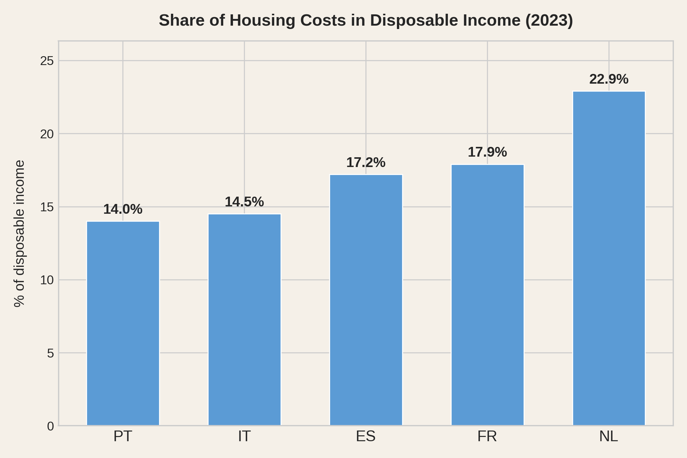
Eurostat publishes exactly such a measure. The EU-SILC survey asks households across Europe what they spend on housing - rent or mortgage interest, utilities, insurance, maintenance, taxes - and reports the total as a share of disposable income. Here is what it says for the five countries featured in this analysis.
At first glance, this looks like exactly the data we need. It isn't.
This is a country-level average. It flattens the extreme regional differences that define the European housing problem - the gap between Lisbon and Beira Baixa, between Paris and the Massif Central, between Amsterdam and Groningen. And Eurostat does not publish this indicator at any finer level of geography.
Worse, the statistic counts rents and mortgage interest but not mortgage repayment. A household paying €1,500 a month on a mortgage - of which €400 is interest and €1,100 is principal - shows up as spending €400 on housing. The other €1,100, the part that actually hurts, is invisible. And the split between interest and principal depends on the rate, the country, and when the contract was signed - making cross-country comparison unreliable even before we consider that countries have very different shares of owners and renters.
The result is a ranking that should give anyone pause. Portugal - a country going through a severe housing crisis - appears as the least burdened. The Netherlands, where the housing debate is real but less acute, appears as the most. The indicator counts rent in full but only the interest part of a mortgage, so its result depends heavily on how each country's households are split between renters, owners with a mortgage and outright owners - and, among mortgaged owners, on how much of each payment is interest. In Southern Europe, where outright ownership is common, a large share of households contributes no rent or mortgage cost to the average.
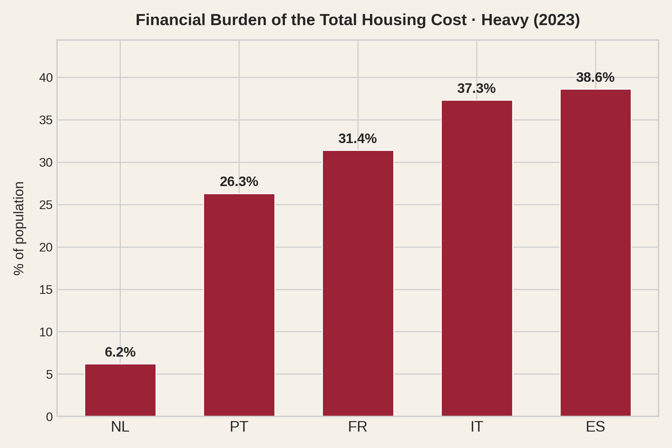
Eurostat publishes a second indicator from the same survey: the financial burden of housing cost, where households themselves report whether housing is a heavy burden, some burden, or no burden at all. This indicator is sensational, in the sense that it measures sensations.
When you ask people how they actually feel, the ranking is very different - and the Netherlands moves from one extreme to the other. Only 6% of Dutch households report a heavy burden. In Portugal it is 26%, in Italy and Spain nearly 40%. The calculated statistic and the lived experience point in different directions.
In our analysis we will study regional differences, face mortgage repayments as what they are - a burden - and avoid relying on sensations to draw conclusions. Using metrics built from actual regional data, we will find all these five countries, and their NUTS-3 regions, in positions that better reflect the economic strain linked to dwelling.
Welcome to the European housing data crisis.
"The first casualty when war comes is truth" - a line often attributed to US Senator Hiram Johnson in 1917. Housing crises have their own version: the first casualty is data. You cannot measure a problem for which there is no objective data.
We have already seen how the best available Eurostat indicator - the housing cost burden - produces a ranking that contradicts lived experience. But the problems run deeper. Europe has no comparable, cross-country dataset of housing prices per square metre. It has no harmonised regional wage data at the level where people actually live and work. To build the analysis you are reading, we had to stitch together data from five different national statistical offices - INE in Portugal, INE in Spain, INSEE in France, ISTAT in Italy, CBS in the Netherlands - each with its own methodology, coverage, granularity and reporting lag. Some publish transaction prices; others publish appraisal values. Some report wages at the NUTS-3 level; others only at NUTS-2, requiring workarounds that introduce uncertainty.
Eurostat, the EU's own statistical office, does publish a European House Price Index. It sounds exactly like what you'd need. It is not. The HPI is an index - it measures how much prices changed within each country relative to a base year (2015 = 100). It can tell you that Portuguese prices rose 89% since 2015. It cannot tell you what a square metre costs in Lisbon versus Madrid. You cannot divide an index number by a wage to get affordability. The one EU-wide housing statistic is structurally useless for the one question citizens actually ask: can I afford to live here?
Mapadomo comes to the rescue. "granular housing data for Europe", they promise. The dataset, with data for 2000-2020, is unavailable (as of November 2026).
Then there is the question of knowing where people actually live. Some countries maintain continuous population registers - the Netherlands and Spain update theirs yearly, France has run a rolling annual census since 2004, and Italy has had a permanent census since 2018. But even these registers struggle to track sub-national migration in real time. In Portugal, which still relies on a traditional decennial census, the president and the national statistics office have had a public debate over whether the official population figures reflect reality. A housing policy that cannot track where people actually live is steering blind.
Throughout this analysis, we use regional employment as a proxy for the number of people economically active in a region. Employment data is updated yearly and registered at the workplace, not the residence. It still undercounts - informal workers leave no statistical trace - but it tracks reality better than population figures that lag behind internal migration. In Southern Europe especially, people can hold formal jobs and pay rent in regions where they have no residence permit. The employment register captures at least part of what the population register misses.
Curating comparable price and wage transaction data across member states is exactly the kind of work the European institutions exist to coordinate. They have the mandate, the staff and the budget. Meanwhile, the analysis you are reading - built from raw national sources, cross-referenced and harmonised at the NUTS-3 level for 312 regions - was assembled by a single citizen, working for free, on evenings and weekends. If one person can do it, the absence of an official equivalent might be a political decision. Or is it the inertia of not deciding? Hard to tell.
Transparency is not about data not being secret. It is mostly about data being available at a reasonable effort. The effort to compare regional affordability does not seem reasonable. This text stems from very unreasonable amounts of effort.
To be fair, they did define the NUTS-3 regional classification and they keep employment data updated. While insufficient for illustration of the present housing crisis, both have been useful for this analysis. We cover 312 NUTS-3 regions across five countries; of these, 309 have both price and wage data for the effort calculation, and the combined scatter plots show 306 because four Paris-area départements are merged into a single data point.
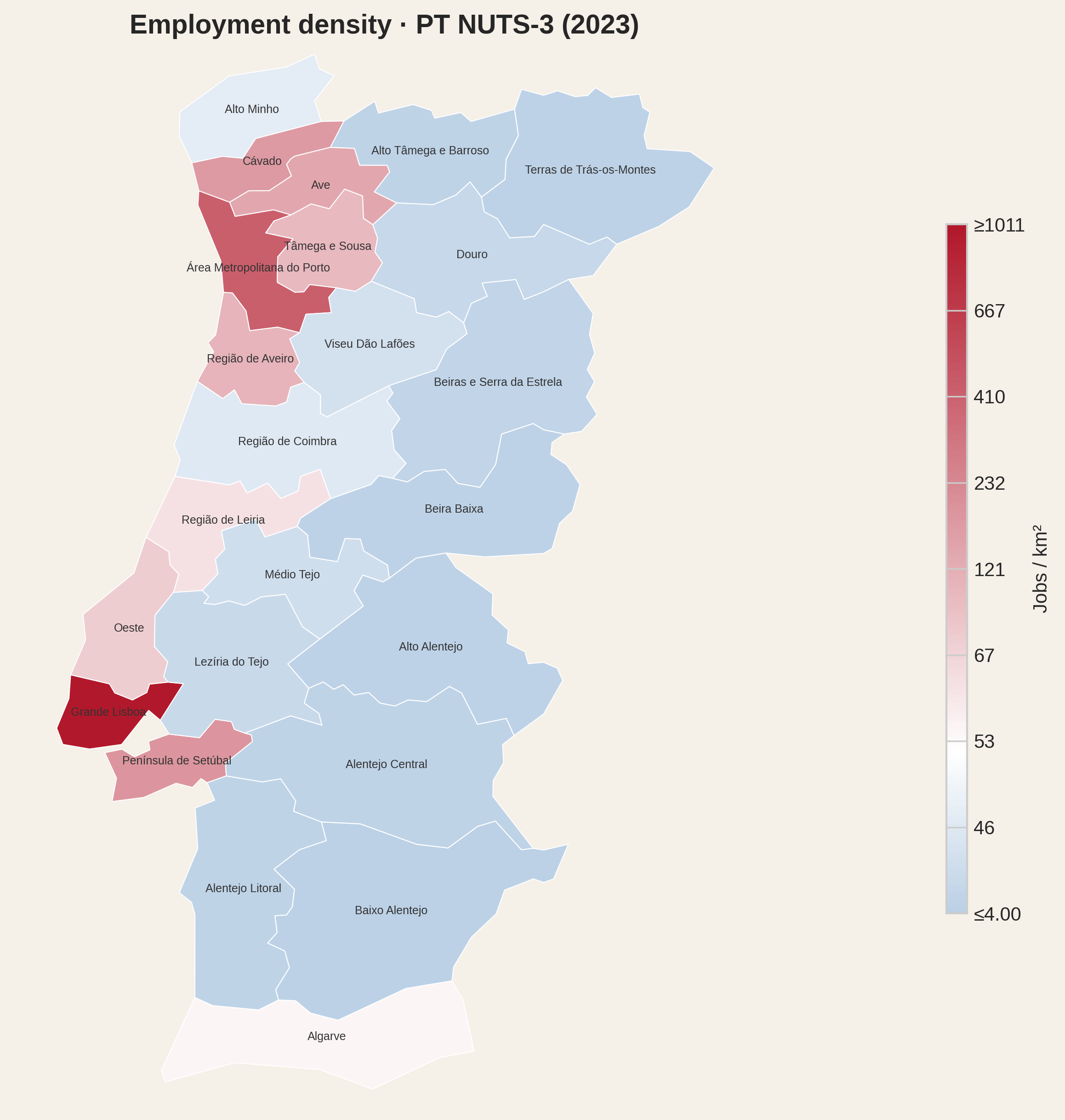
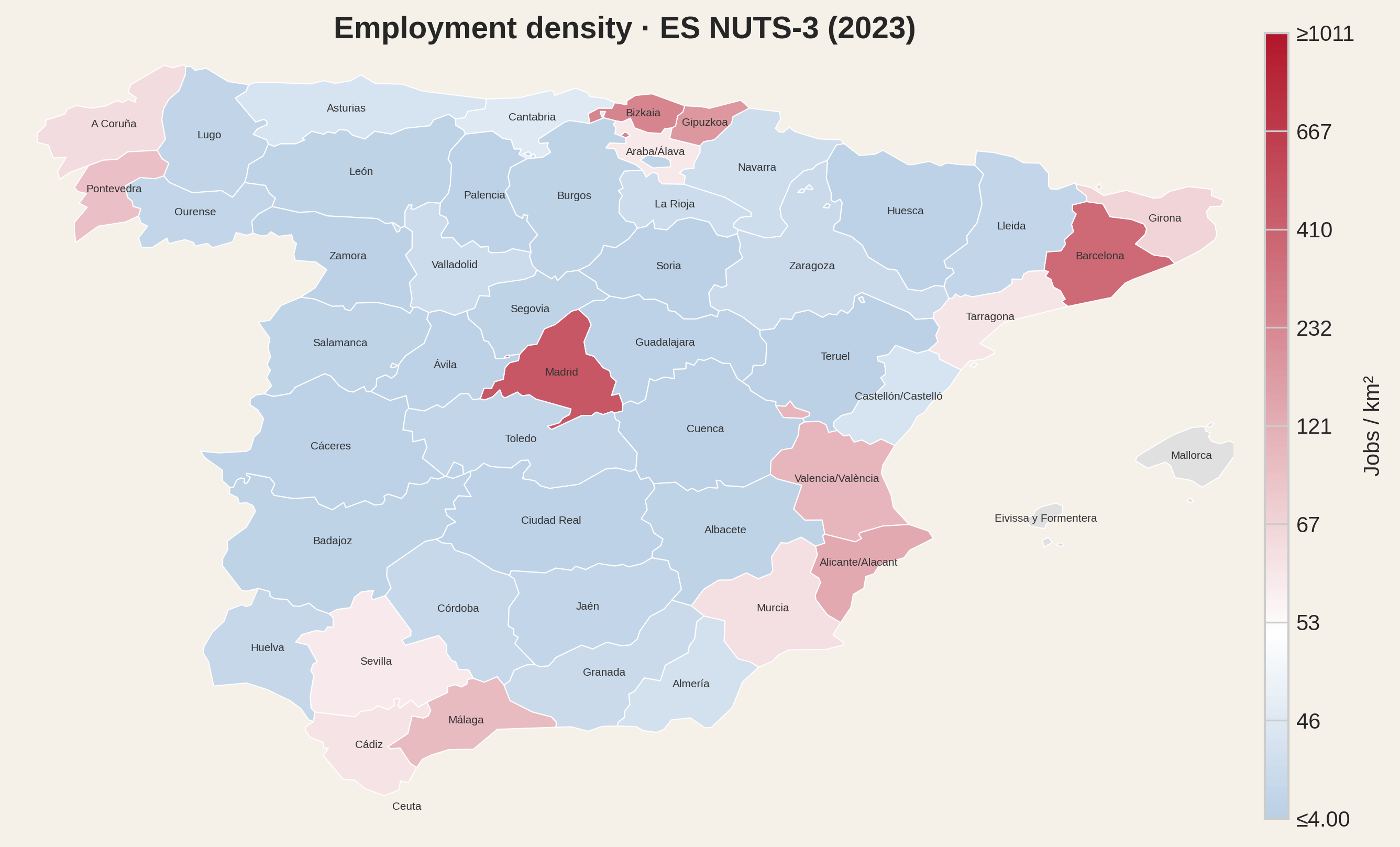
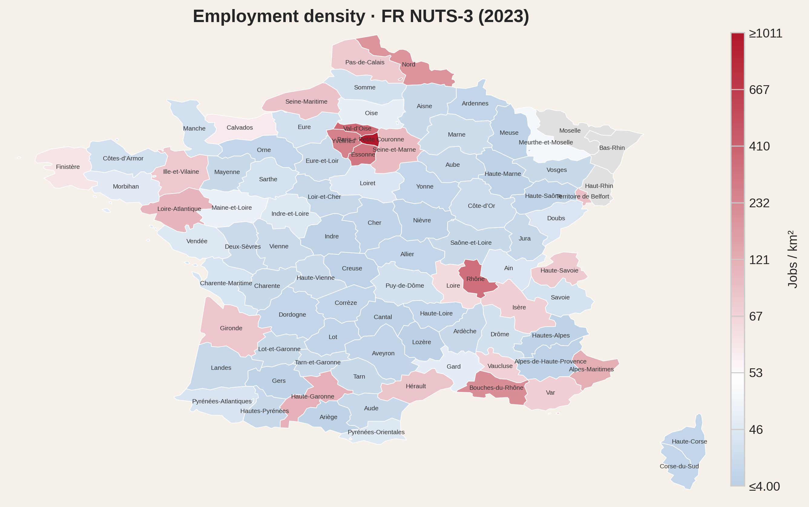
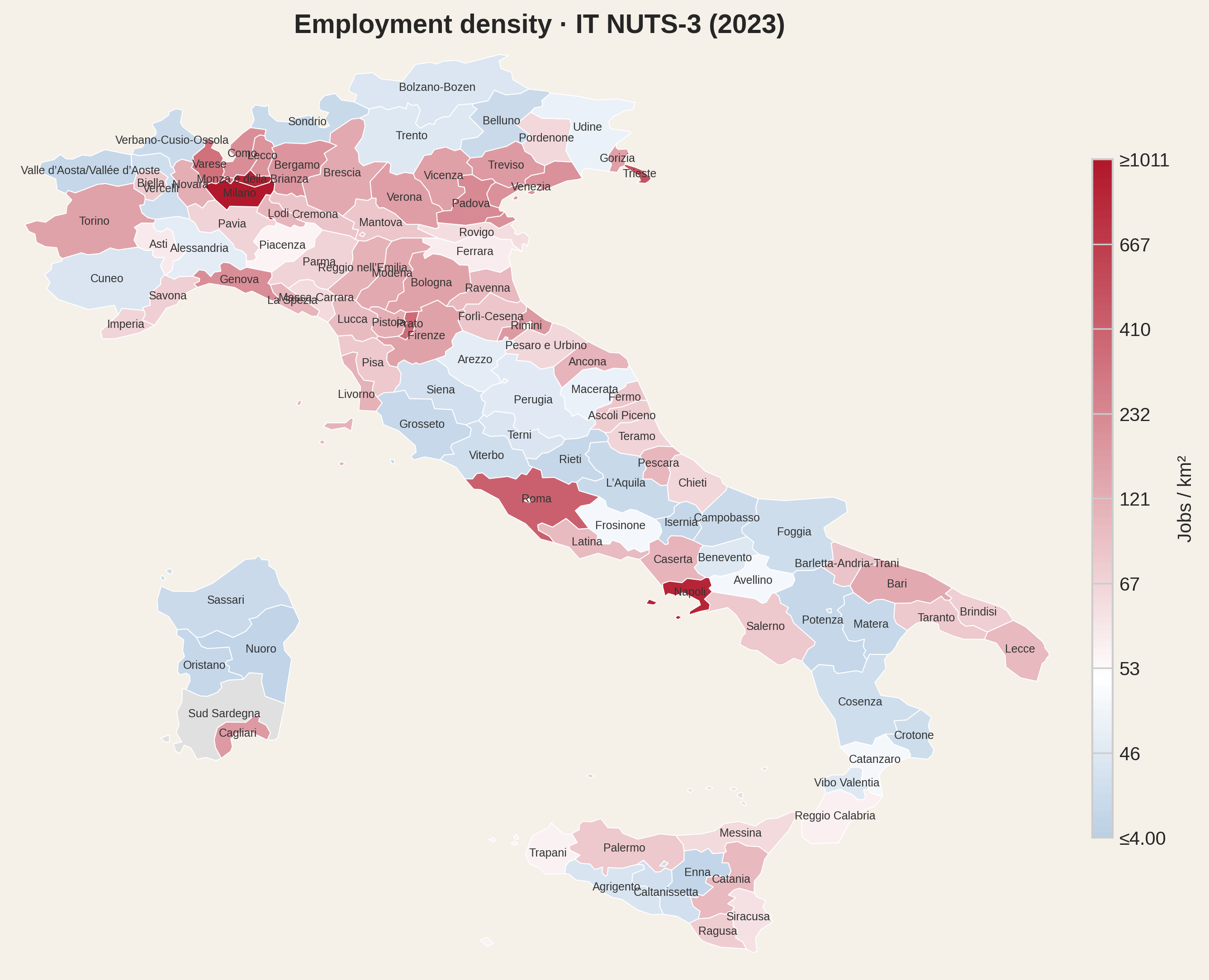
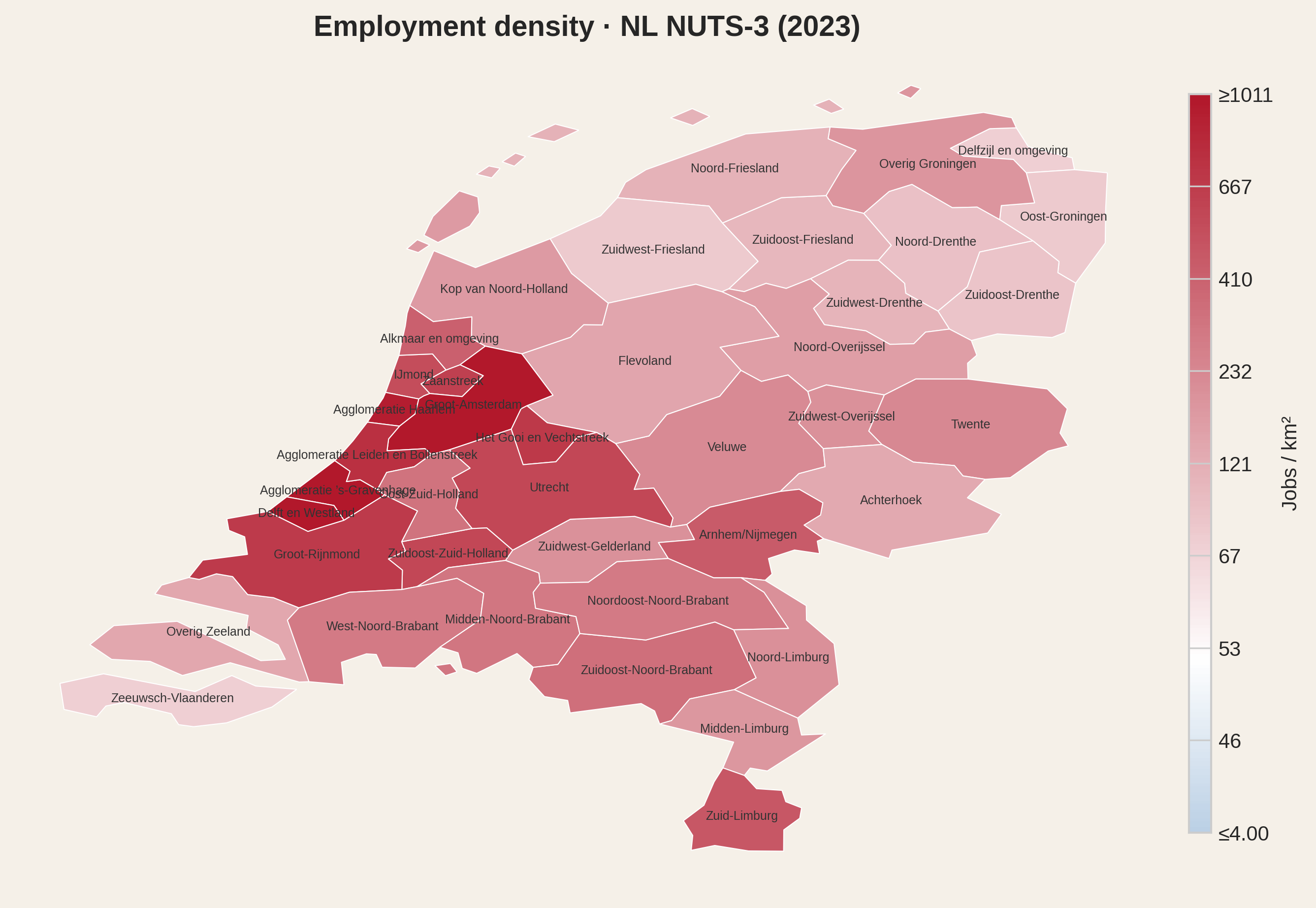
Before looking at prices and wages, it helps to see the landscape they operate in. Employment density - the number of jobs per square kilometre - is the simplest measure of economic activity. The maps below show it for all NUTS-3 regions in our dataset. White marks the median density across all regions; blue runs toward the sparsest provinces, red toward the densest.
Portugal
Spain
France
Italy
Netherlands
The pattern is immediate. Jobs cluster in a few places: the Lisbon-Porto coastal strip, the Madrid-Barcelona axis, the Île-de-France blob and its Lyon-Marseille satellites, the Po Valley running from Turin to Venice. The interior is pale. In Portugal, a worker in Grande Lisboa has a thousand employed people per square kilometre around them; in Beira Baixa, ten. That is not a subtle gradient but a rather different economy. The Netherlands is overall more uniform and more job-dense.
This is the map that housing prices have to be read against. A region's affordability only makes sense relative to whether anyone can actually work there.
A square metre in Lisbon costs less than a square metre in Amsterdam. But does that make Lisbon more affordable? Only if the person buying it earns a Dutch salary.
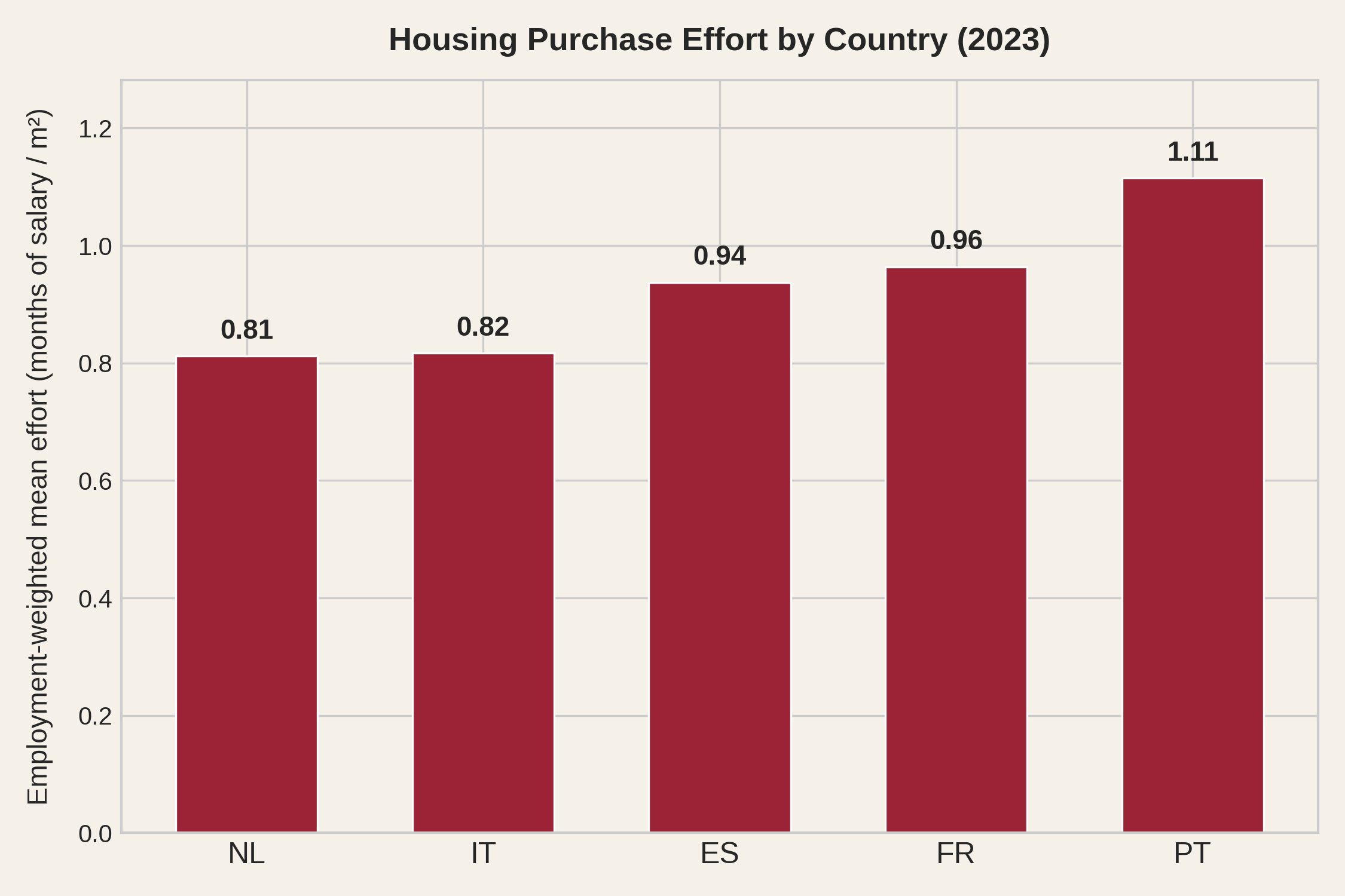
Let's divide the price of the square meter in a region by the wage of that region, using means or medians, depending on what statistic is available. We call this metric housing purchase effort: the number of months of gross salary needed to buy a single square metre. Because it is a ratio of two local quantities measured in the same currency, it allows direct comparison across regions and years, eliminating the problematic effects of regional wage differences and inflation. At the national level, the picture is already telling.
Portugal and France look remarkably similar - around one month of salary per square metre. The Netherlands, despite far higher prices, comes out better because wages more than compensate.
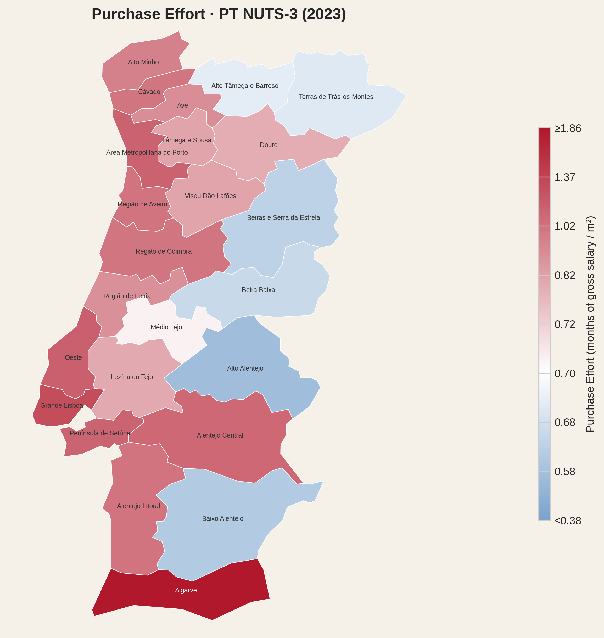
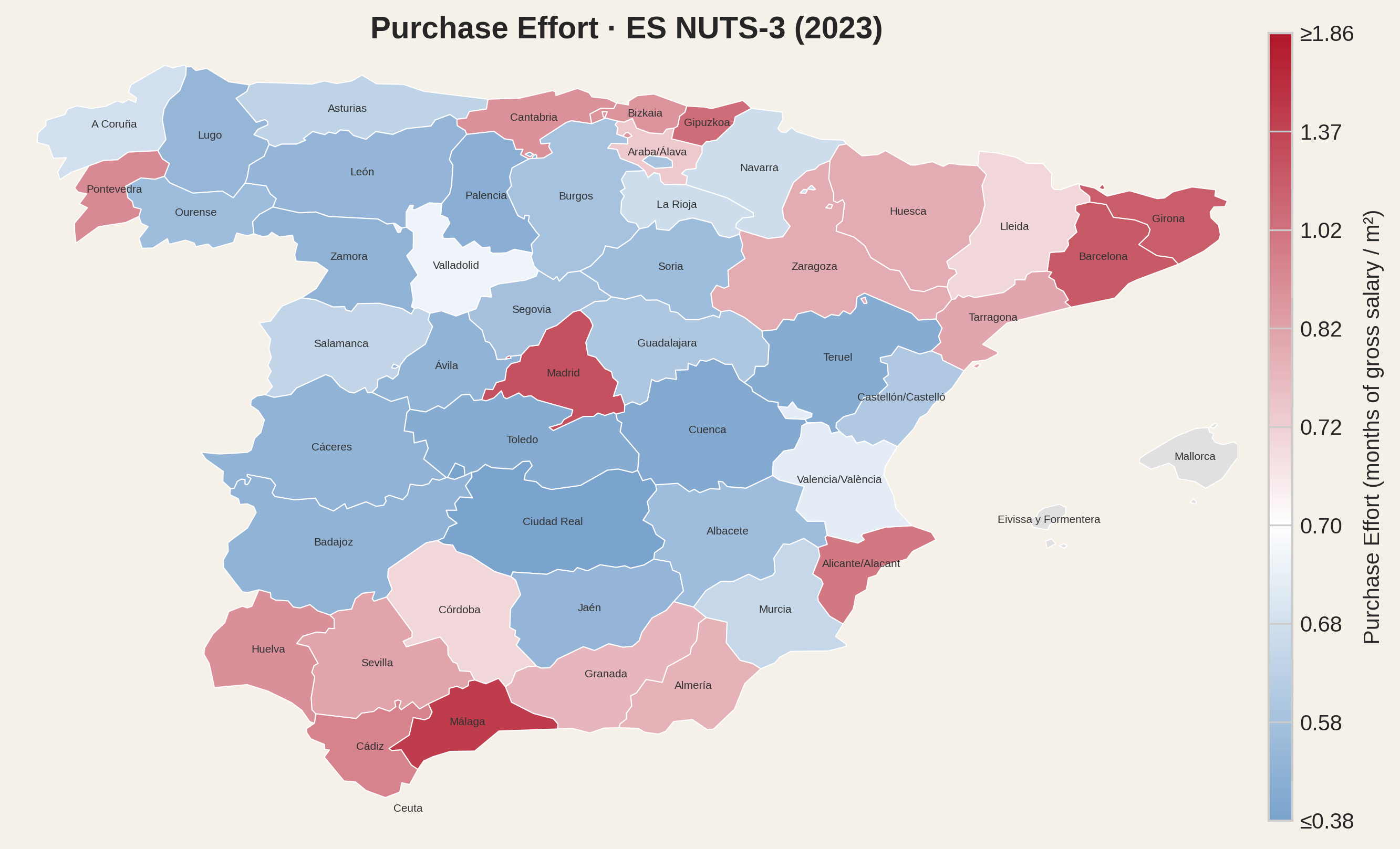
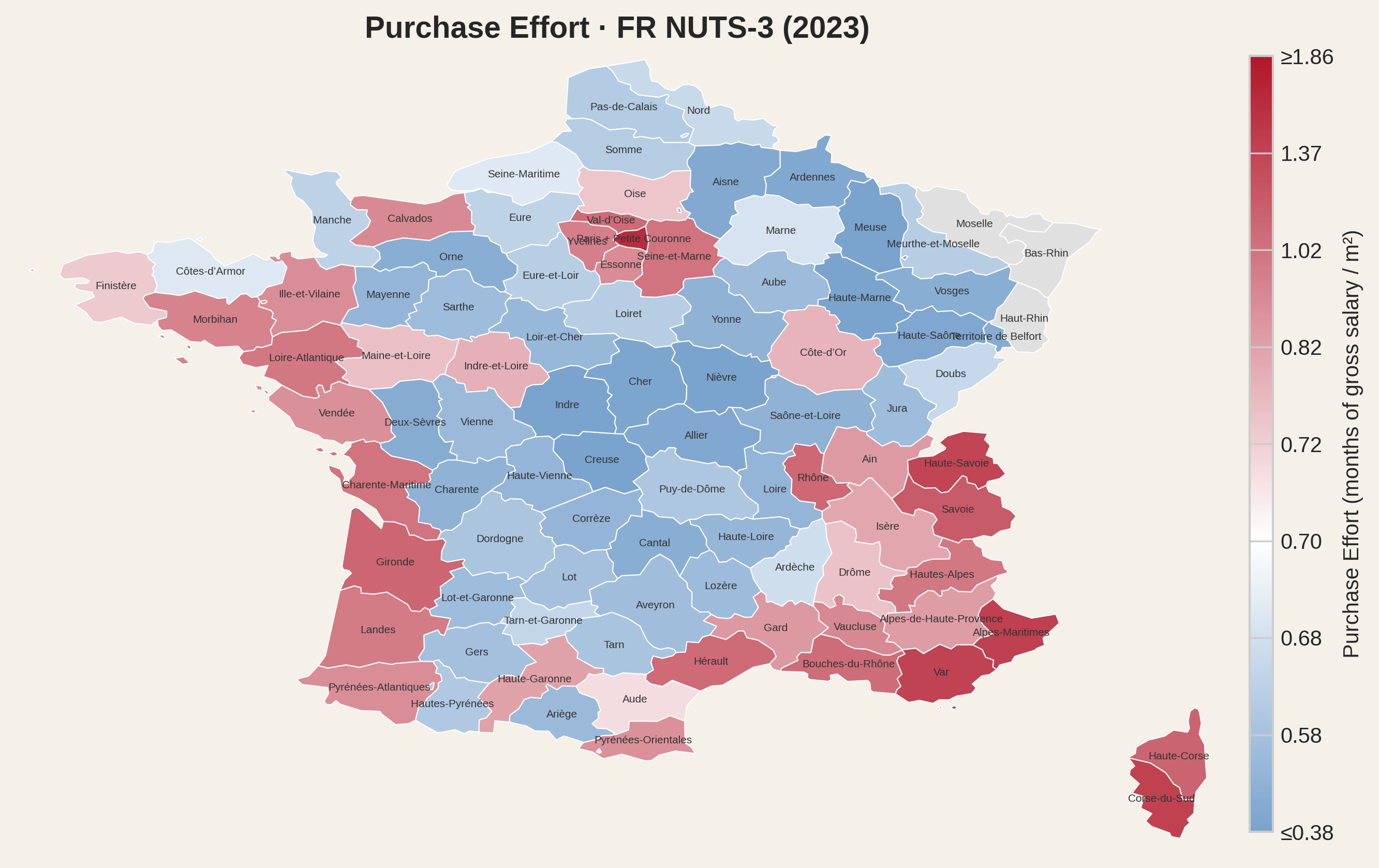
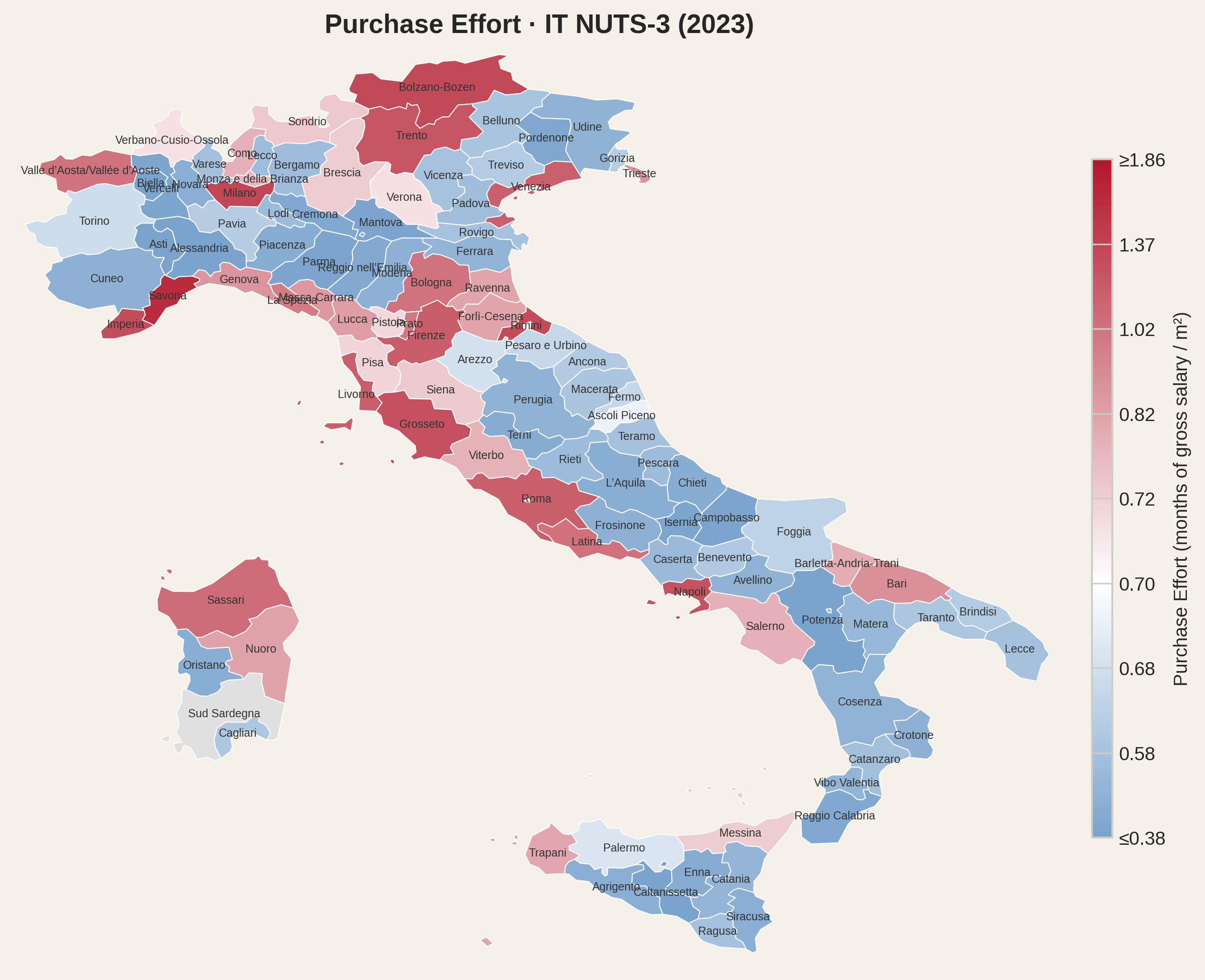
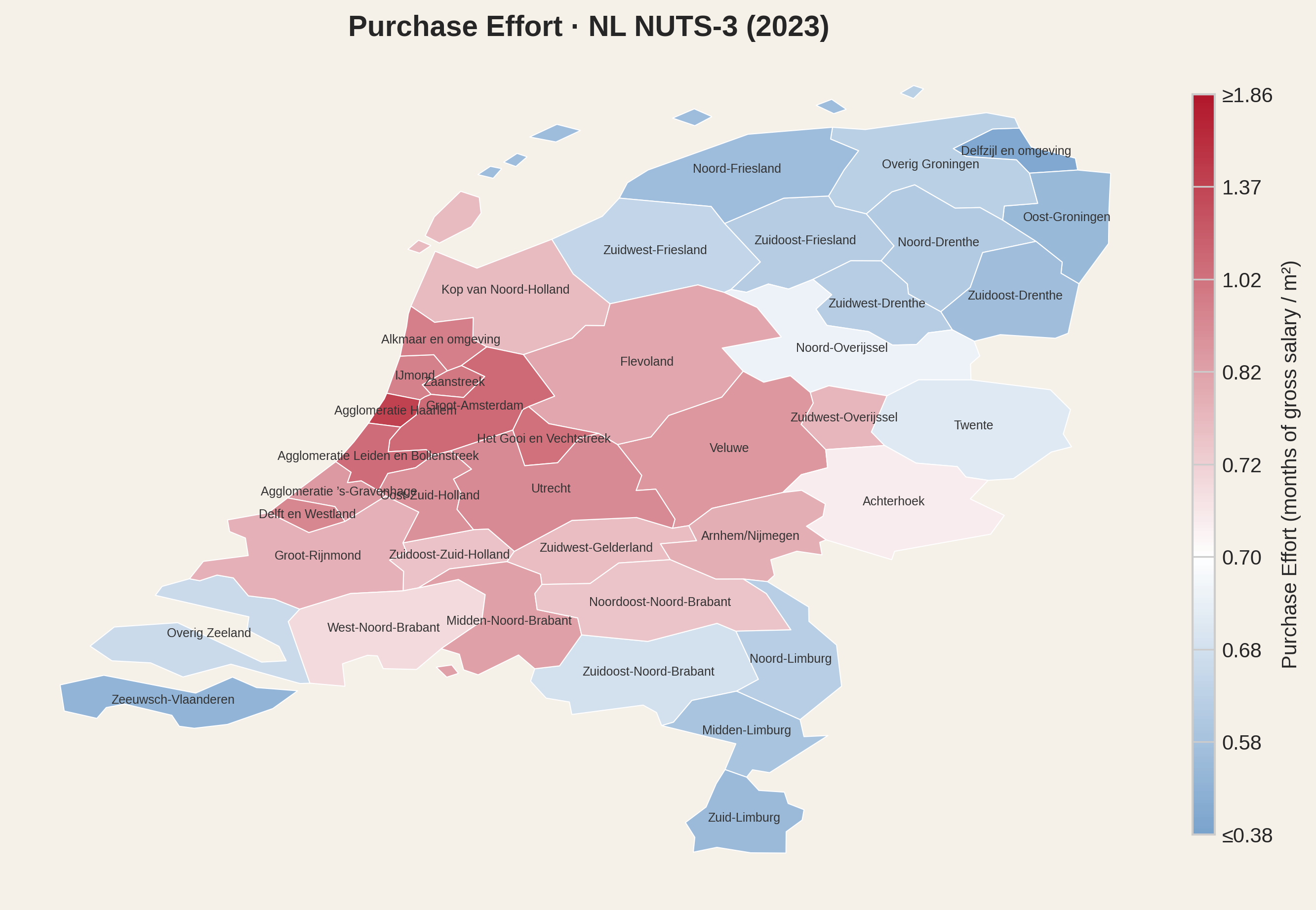
These are national averages. The real story appears when we zoom in to NUTS-3 level - the smallest regional unit for which both housing prices and wages are available. White on the map marks an effort of 0.7 - roughly the threshold at which a 50 m² apartment can be repaid in about ten years at maximum mortgage effort. More on loan repayment in Part eight.
Portugal
Spain
France
Italy
Netherlands
The maps reveal what national averages hide. Within a single country, the variation in effort is often larger than the variation between countries. A worker in the Algarve faces a fundamentally different reality than one in Bragança - same country, same labour law, but wildly different affordability.
What explains the variation? House purchasing effort reflects a demand-supply relationship: when more people compete for limited housing stock, prices rise relative to wages. To lower effort, a region needs more houses per resident. But building more is not always possible - you cannot upgrade buildings from 10 to 20 floors once they are built, and widening a road from four to six lanes does not help if single-lane bottlenecks lie between commuting points. Even when possible, building takes a long time. Population relocation or inflow can happen much faster than supply adjustment, which requires projects, permits, manpower and bricks. Because of this, regions that face continuous increase of demand may never fully adjust - they become dense under constrained supply.
It is worth saying that density brings efficiency up to a point, not indefinitely and not regardless of case-by-case circumstances.
Neither housing supply nor actual demand are reliably measured at the regional level - another data gap. What we do have is employment density: employed persons per square kilometre. In regions that are not overly touristic, this is a reasonable proxy for demand pressure on housing.
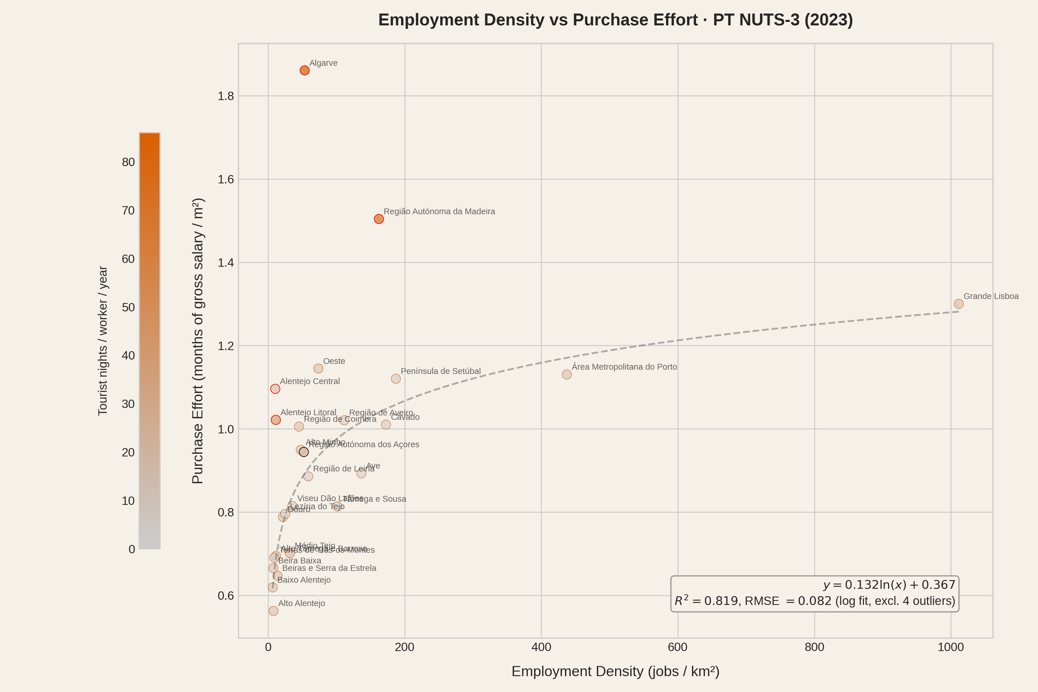
When we plot employment density against purchase effort, a pattern arises: denser regions are systematically harder to afford.
Portugal has only 26 NUTS-3 regions. Azores uses a NUTS-2 wage fallback because national wage data is unavailable for this region; plot captions give the number of regions shown, but fallback regions are excluded from the regression fits throughout. A log-linear fit to the 25 non-fallback regions explains 33% of the variation in effort (R² = 0.33). That rises to 82% when we set aside four outliers - Algarve, Madeira, Alentejo Litoral and Alentejo Central - regions where tourism and/or other local factors push effort well above what density alone would predict. Outliers are marked with a red circle in the plot. Colour saturation encodes tourism intensity (overnight stays per worker) - the more saturated the dot, the higher the tourism pressure.
Portugal (26 regions)
With a sample this small, a handful of regions can move the fit substantially, so the R² should be read with caution. Still, the direction is unambiguous: denser regions come with higher purchasing effort.
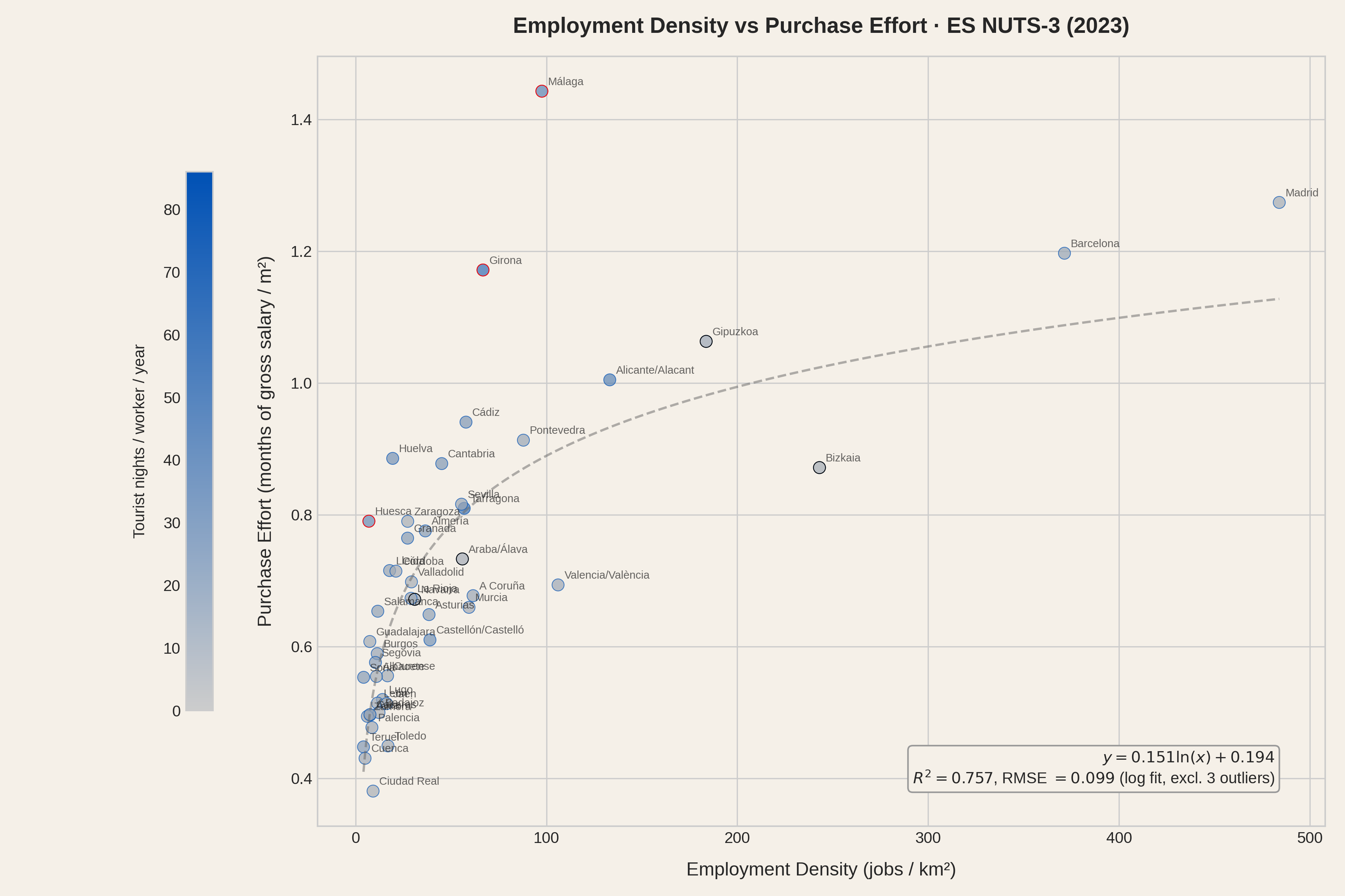
Spain provides a larger sample: 47 of its 59 NUTS-3 regions. The missing twelve are the Balearic Islands, the Canary Islands, and the autonomous cities of Ceuta and Melilla, where price or wage data is not available at this level of geography. The four foral provinces (Álava, Bizkaia, Gipuzkoa, Navarra) are included but use NUTS-2 fallback wages, since AEAT does not cover territories with their own tax administrations; these four are excluded from the regression fit, leaving 43. Density alone explains 64% of the variation, that value rising to 76% (R² = 0.757) by excluding touristic outliers Málaga and Girona, and a third outlier called Huesca. The larger sample, with a lower proportion of outliers, allows for a more stable estimate of the relationship.
Spain (47 of 59 regions; islands and autonomous cities excluded).
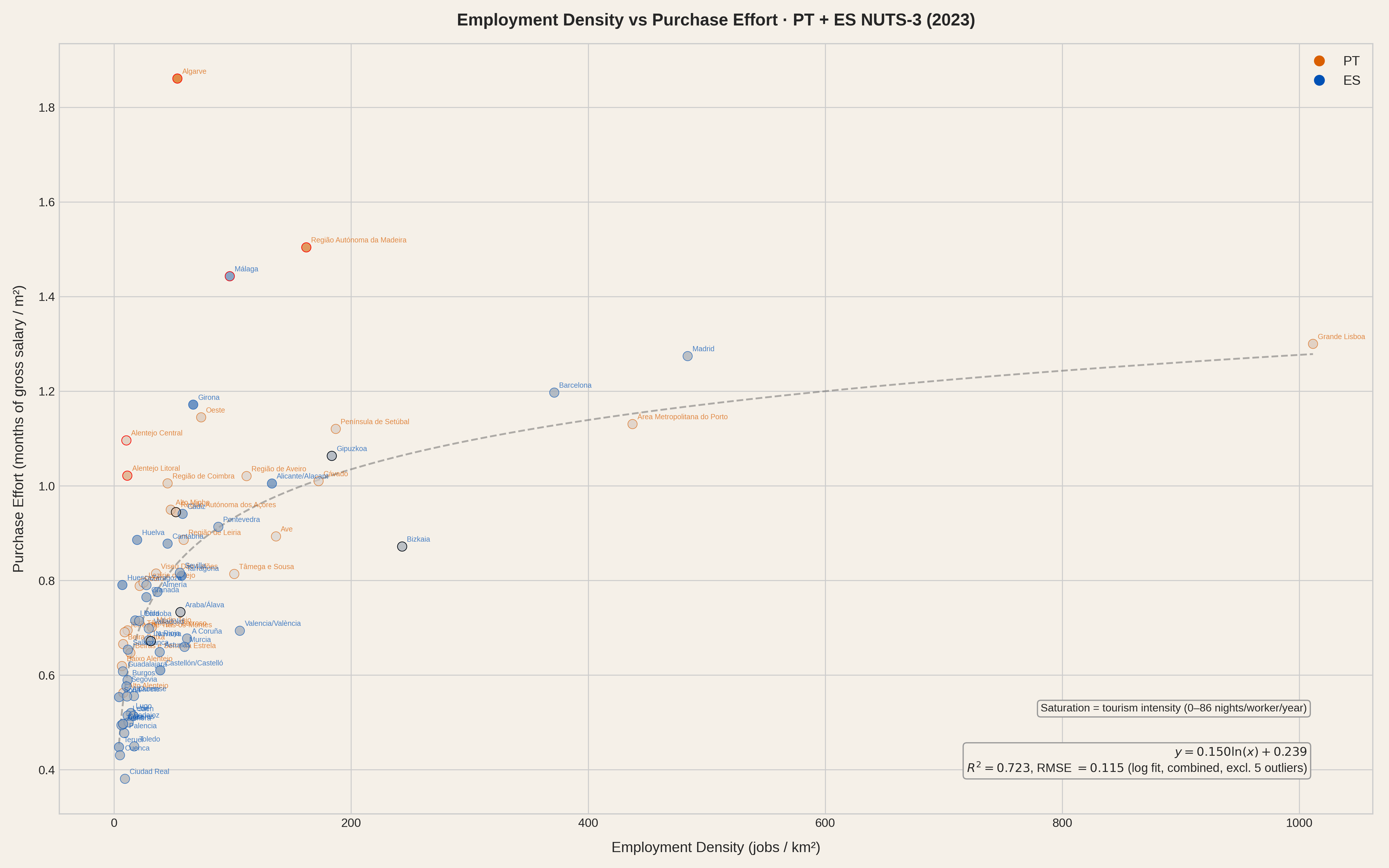
When we pool Portugal and Spain together - two countries with very different wage levels, price structures and regional geography - the combined sample reaches 73 regions (68 after excluding fallbacks). Density alone explains 50% of the variation (R² = 0.50), rising to 72% when we exclude the five outliers of this combined fit (Algarve, Madeira, Alentejo Litoral, Alentejo Central, Málaga). The relationship survives crossing borders.
Portugal and Spain combined (73 regions). Two different countries, one pattern.
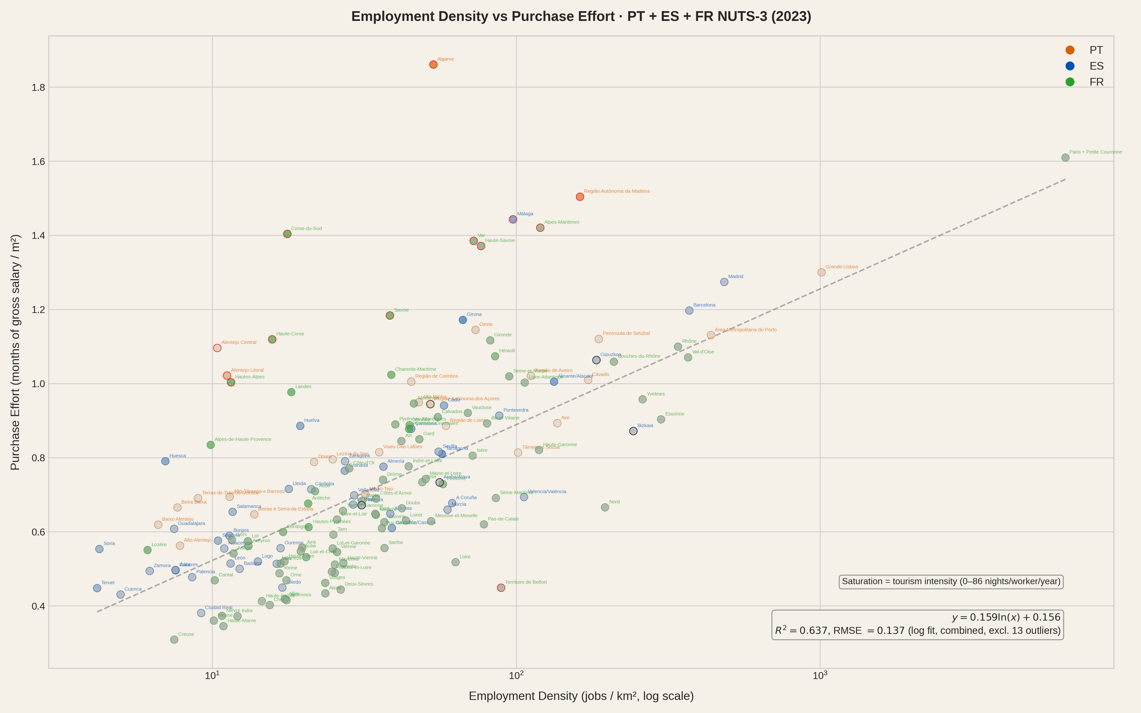
Adding France brings 90 of its 96 metropolitan départements. Three are missing because the DVF property transaction database does not cover Alsace-Moselle (Bas-Rhin, Haut-Rhin, Moselle), where a local land registry law predates the national system. The remaining gap is Paris: its NUTS-3 boundary covers only the 103 km² city proper, registering over 21,000 jobs per km² - a density so extreme it compresses every other region to the left of the chart. To make Paris comparable to other capital regions we merge it with the three départements of its Petite Couronne (Hauts-de-Seine, Seine-Saint-Denis, Val-de-Marne), weighting by employment. The merged Paris metro unit still leads the density ranking at around 6,500 jobs/km², but the effort index drops from 2.1 to 1.61 - high, but no longer on a mathematical cliff. This is also why we switch to a logarithmic x-axis: even after merging, the density range spans from single digits to thousands. This merge is not cheating: data work is sometimes messy and the NUTS-3 classification is not clean either (see NUTS-3 regions are not equal in the appendix).
With 163 regions across three countries (158 fitted), density explains 64% of the variation in effort (R² = 0.637, excluding 13 outliers). The logarithmic relationship holds across borders, wage systems and housing markets.
Portugal, Spain and France combined (163 regions, Paris merged with Petite Couronne). Log scale.
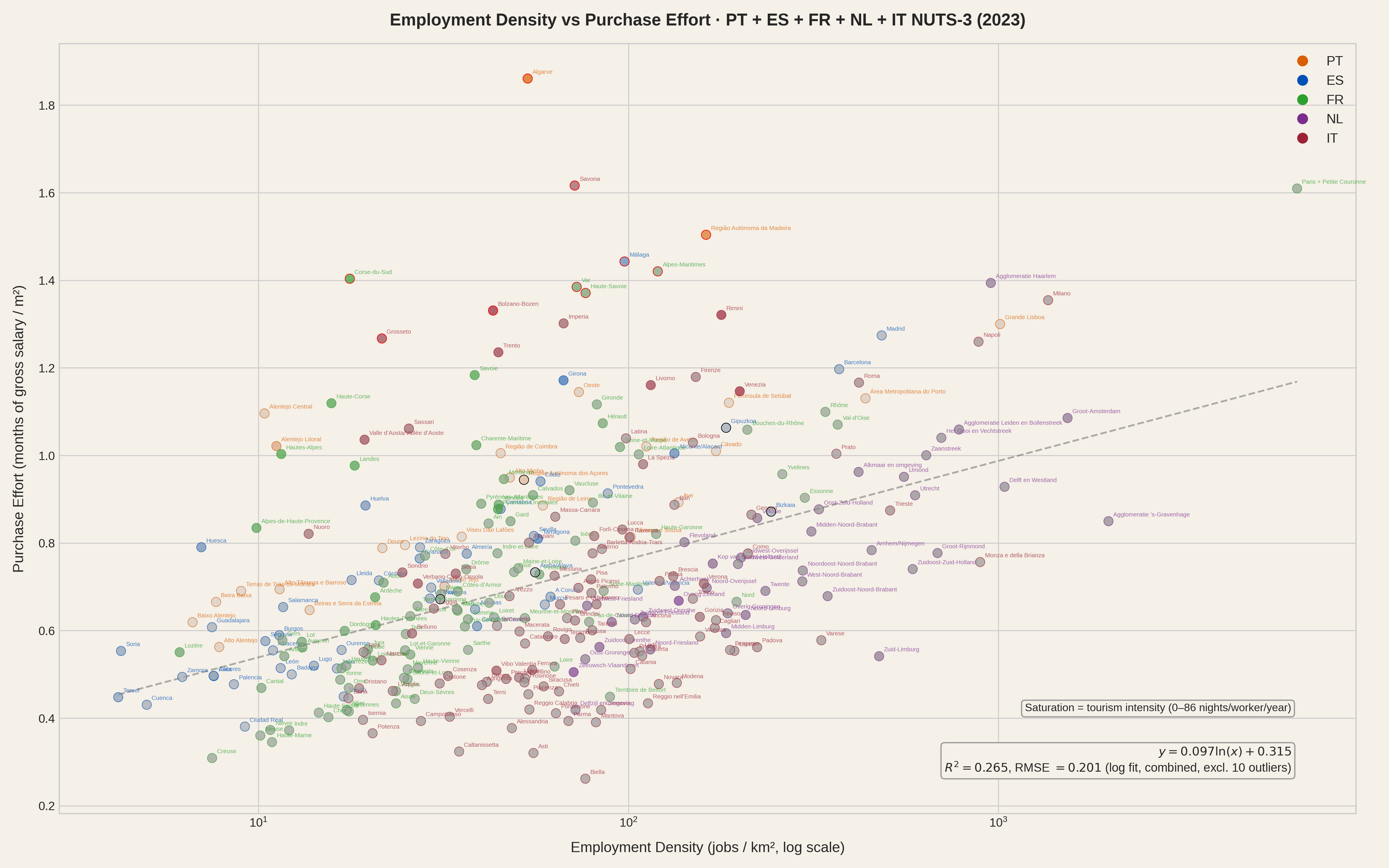
And it still holds directionally with all five countries combined, despite the complexity of Italy, the unusual affordability of the Netherlands relative to its job density, and the existing comparability issues (see Comparability caveats in the appendix).
All five countries (306 regions, Paris merged with Petite Couronne). Log scale.
The easy reading of this data is "large cities are expensive." Certainly, prices rise with job density and so do wages. But wages in dense areas don't rise proportionally to housing costs. The gap between what housing costs and what people earn widens as you move toward the economic centres. Then there are the obviously touristic regions: Algarve, Málaga, Girona, Alicante, the Côte d'Azur (Alpes-Maritimes, Var), Corsica, Rimini, Bolzano. These regions are low density, high effort - tourism inflates prices where local wages, driven by a non-touristic job market that is not competitive enough, have no chance of keeping up. These regions are a very specific minority where what happens does not follow the general rule. And they are usually not the ones that include the capital.
Removing these outliers reveals a strong density-effort relationship that holds even when mixing several countries. It does not remove the effect of tourism - it removes the effect of extreme tourism. The regions that remain still feel tourism to varying degrees, and that residual influence partly explains why the fit, while robust, is not perfect: moderate tourism pushes some regions above the density-only trend line without being extreme enough to flag them as outliers. Once we recognise this, the natural next step is not to keep discarding data points but to accept tourism intensity as a second variable alongside employment density.
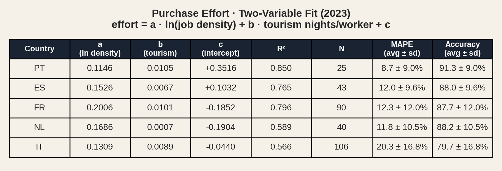
A multivariate model using only two predictors - employment density and tourism intensity - explains 57% to 85% of the variation in effort, depending on the country.
Model: effort = a·ln(density) + b·tourism + c. Tourism measured as overnight stays per worker.
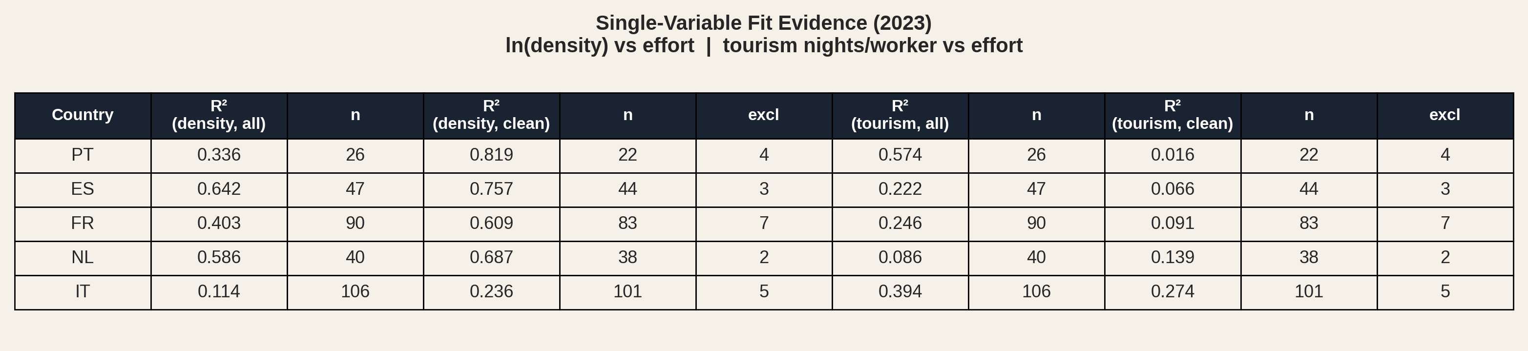
We can isolate each variable's contribution by fitting for density and tourism separately. The table below shows R² for density-only and tourism-only fits, both with all regions and after excluding outliers.
Single-variable OLS fits: ln(density) vs effort and tourism nights/worker vs effort. "Clean" excludes IQR-detected outliers.
Density alone explains 34% to 64% of the variation, rising to 61% to 82% after excluding outliers - the touristic regions that break the density pattern. Tourism-only fits tell the opposite story: R² stays below 0.25 for Spain, France and the Netherlands, and the already low values collapse further after outlier exclusion. Portugal's tourism-only R² of 0.57 is driven by the strong pull of a few touristic outliers like Algarve and Madeira - small samples (n=25 fitted) make such anomalous situations more likely; once those outliers are removed, tourism explains essentially nothing (R² = 0.02). Italy is the exception: tourism-only R² is 0.39 with a large enough sample (n=106) to make accidental alignments unlikely, and it holds at 0.27 after outlier exclusion.
Unlike fitting for density, fitting for tourism alone does not expose a small number of outlier regions that could be removed to improve the fit. That's because, apart from Italy where the situation is more complex, tourism-driven regions are the exception, easily identified as outliers when fitting for density.
Comparing the two tables confirms this reading. The multivariate fit (density + tourism) improves on the density-only fit in every country - tourism always adds predictive power. More telling: the multivariate fit also beats the density-only-clean fit (outliers excluded) in four of the five countries. Even after removing the most touristic regions, the result is worse than with tourism as a second variable. The single exception is the Netherlands, which makes sense: it is not a tourism-heavy country, and its outliers are likely driven by other factors.
The takeaway: in most regions, tourism modulates the influence of job density - it nudges effort up or down around a trend that density sets. Only in a handful of regions does tourism override job density entirely and become the dominant force.
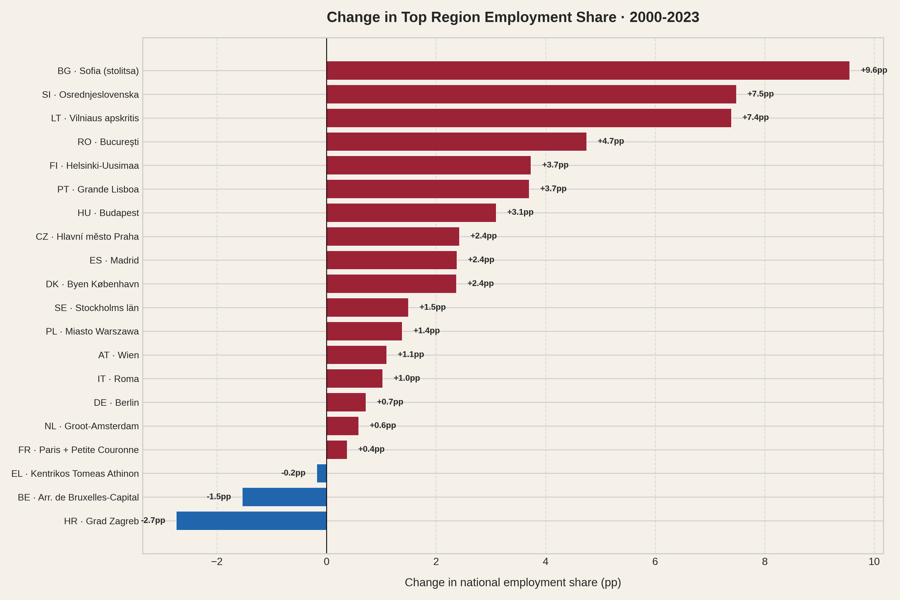
Capital regions concentrate a disproportionate share of national employment. Grande Lisboa alone holds 25.5% of all jobs in Portugal. Madrid holds 17.9% of all jobs in Spain, the Paris metro (Paris + Petite Couronne) 15.9% in France. Even in polycentric Italy, Roma accounts for 8.5%, matched only by Milano at 8.2%. Workers do not choose these regions on a whim - they go where the jobs are.
And the jobs are expensive to live near. Capital regions rank among the highest in effort - the Paris metro reaches 1.61, Grande Lisboa 1.30, Madrid 1.27, Groot-Amsterdam 1.09 - driven by the density relationship we have seen: more workers competing for housing in a bounded territory. Tourism-heavy regions like the Algarve (1.86) or the Côte d'Azur (1.42) can rank even higher. To make this concrete, we translate effort into mortgage repayment time for a 50 m² flat.
These are regions where a single earner needs nearly two decades or more to repay a modest flat. Even after combining four départements, the Paris metro requires 37 years. A 75 m² apartment instead? The monthly payment no longer covers the interest. The loan is never repaid. And these timelines cover only the mortgage itself - saving for the 10% deposit and transaction taxes, which add roughly 3% to 12% of the purchase price depending on the country, is time not included in the simulation (see Part eight).
Paris itself is even more extreme. Its NUTS-3 region (FR101) covers only the dense urban core, where the effort index reaches 2.1 - pushing the mortgage calculation to 101 years. But that number sits on a mathematical cliff: at 4% interest, the monthly payment barely covers the interest on the loan. A small rate increase to 4.2% tips it over the edge - the loan becomes infinite. A drop to 3.5% brings it down to 56 years. No other region in our dataset is this sensitive to assumptions, which is why we lead with the Petite Couronne figure instead.
The trap is not just financial. Capital regions are large enough that living on their edge already means a long commute, and living outside them means commuting even further while inheriting some of the inflated housing prices. Workers in surrounding regions earn wages that do not match the centre but face prices driven up by proximity to it. (See NUTS-3 regions are not equal in the appendix for how boundary size affects cross-country comparisons.)
In public debate, tourism is frequently cited as the primary driver of housing unaffordability. Short-term rentals, foreign buyers, holiday apartments consuming the housing stock. The narrative is compelling and, in specific places, not wrong.
The data tells a different story at scale.
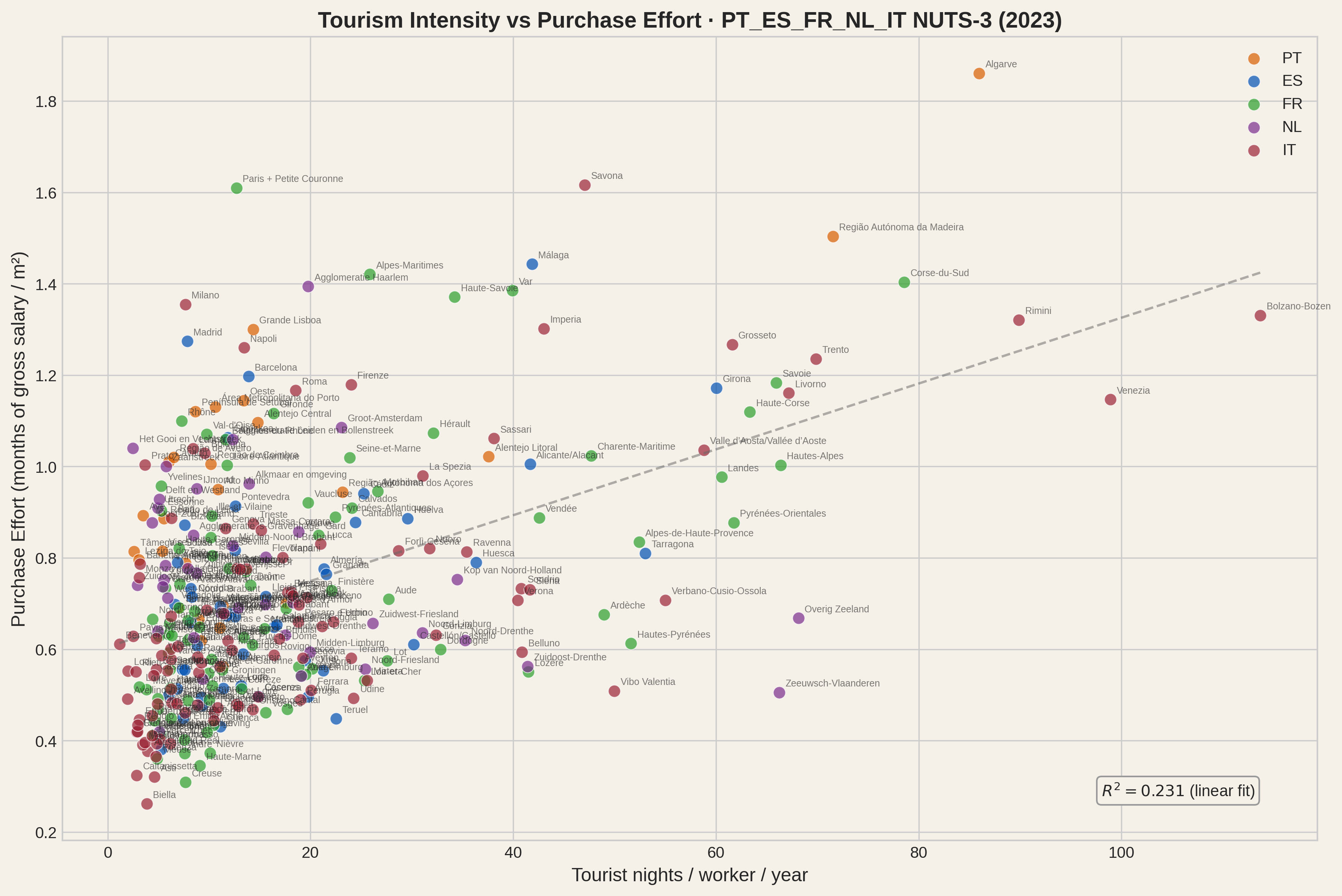
Tourism intensity (overnight stays per worker) vs. housing purchase effort across all five countries.
Tourism does correlate with higher effort - the multivariate model confirms it has a small, positive coefficient in every country. But as a single variable it explains only 23% of the variation across all five countries (R² = 0.231), and as we saw in the single-variable fit evidence, that number collapses for most countries once outliers are removed.
Despite a similar R² (the five-country density vs effort fit has R² = 0.265), this plot is substantially different from the density vs effort plot for all countries: visually, we don't see a way for improving the fit by removing a handful of data points. Unlike what happens with the density vs effort plot where a clear group is identifiable by eye - even if not automatically marked as outliers - removing the oddities here leads to "vertical data", i.e. no correlation.
There are particular regions where tourism has a strong influence like the Algarve, the Côte d'Azur, the Balearics or Corsica. It is also true that some city centres are disproportionately under pressure, with both employment and tourist demand in the same square kilometres. It is even fair to say that tourism intensity should be actively monitored and managed in all the regions - there are other good reasons, apart from house prices.
Still, the contribution of tourism to the overall picture is secondary. Within each country, employment density - the sheer number of jobs per square kilometre - explains far more of the variation than tourism does. And Europe is not facing a city-centre-only crisis. NUTS-3 regions span entire metropolitan areas, suburbs and commuter belts. When a NUTS-3 region is unaffordable, it means that even workers willing to endure long commutes within it cannot escape the cost pressure. The problem covers the territory where people actually live, not just the postcard downtown. The problem of scapegoating tourism is that we may remain blind to the structural problem of density. And risk overshooting tourism restrictions without achieving meaningful results.
Is there a causal relationship between density and effort? Correlation does not imply causation, but it invites analysis.
When job density and effort move together, three readings are possible: effort causes density, density causes effort, or both are caused by something else.
The first is implausible - high housing costs do not attract employers. The third is more subtle: one or more external factors would need to drive both density and effort in such a way that the specific logarithmic relationship we observe between them is produced across different countries. It is not enough for a confounding variable to merely raise both; it would need to shape them into a specific mathematical form. Explanations based on confounding variables (geographic constraints, cultural traits, ...) would require many things to fall in the right place, with the right intensity, across several countries. The reading that best survives parsimony is the most direct: density causes effort because people need to work and tend to live within commuting distance of the workplace. NUTS-3 regions are typically large enough to contain both workplaces and residences. Within a region, prices react to demand pressure more vigorously than wages do, because building houses takes time and accepting a longer loan feels like a better option than not having a job.
Employment density is the candidate structural driver. Tourism amplifies specific hotspots and influences other regions, but it is not the master variable. Companies open offices where talent lives. People move to where they can work. Demand concentrates. Prices rise. More companies open offices where talent already moved. More people move there. The cycle feeds itself.
For some regions, housing is mathematically out of reach under any reasonable set of mortgage assumptions.
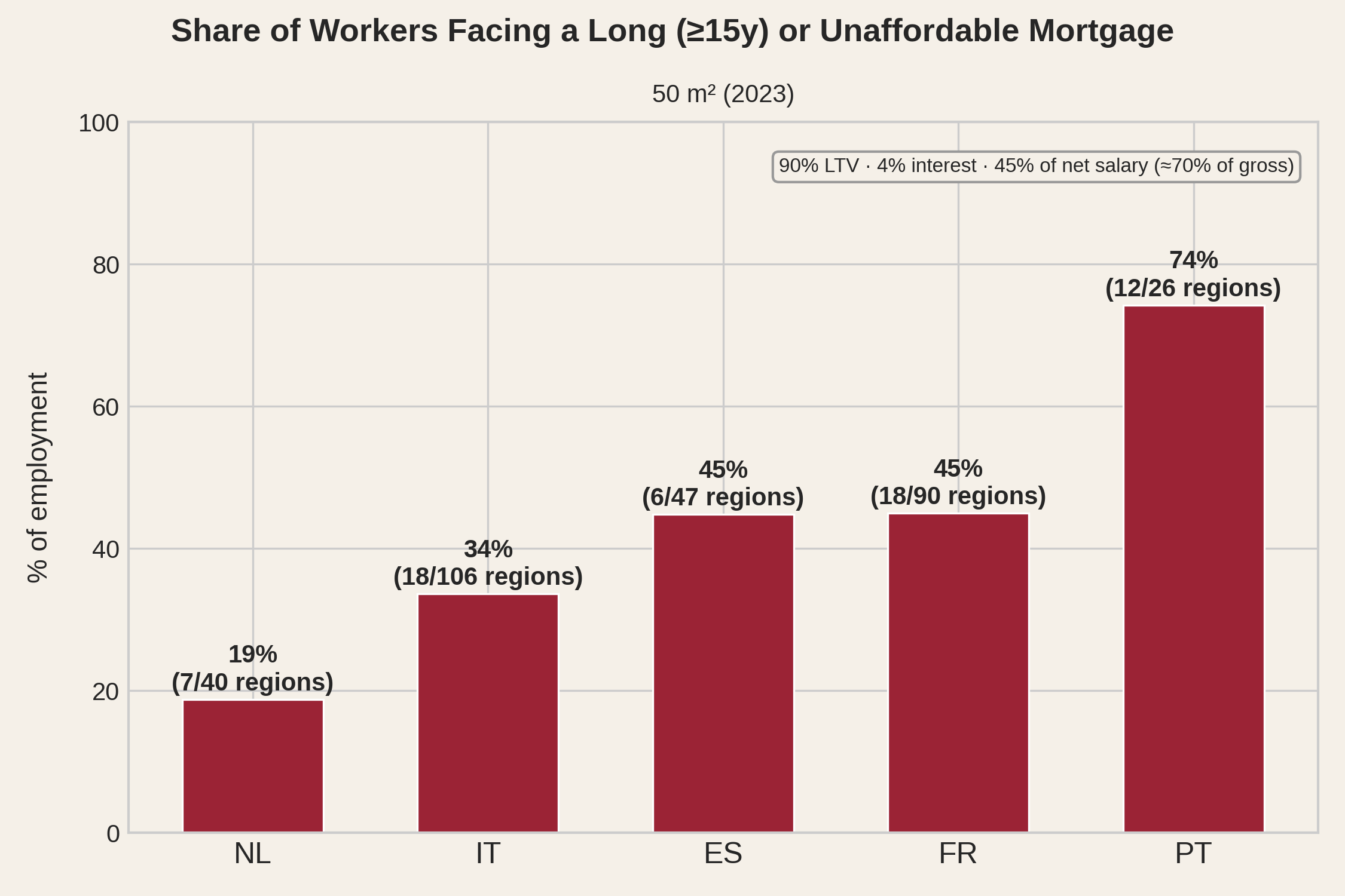
When we simulate a standard mortgage - 90% loan-to-value, 4% interest, 45% of net salary going to repayment - a large share of workers face a repayment period of 15 years or more for a 50 m² flat. This is roughly a studio or small one-bedroom apartment. In Paris and its Petite Couronne, the combined capital region, a 50 m² flat takes 37 years to repay. Paris itself sits on a mathematical cliff where the payment barely covers interest (see Part six). In Lisbon, the simulated average loan repayment for a 50 m² apartment is 24 years.
A 45% effort ratio is unusually permissive. It matches Portugal's regulatory DSTI limit, but exceeds France's 35% limit and the affordability thresholds commonly applied in Spain and Italy. The Dutch system uses income-dependent limits rather than a fixed percentage. The simulation therefore uses a relatively generous assumption, and actual borrowing capacity may be lower.
Furthermore, these figures count only the loan. Before the first payment, a buyer must save the 10% deposit plus transaction taxes and fees - which range from roughly 3% of the purchase price in the Netherlands to 8-12% in Spain and Portugal, with France and Italy in between. Early in a career, when salaries are lowest and savings hardest to accumulate, this can take years. The time required to become a homeowner can therefore extend well beyond the simulated mortgage repayment period.
The simulation pairs one salary with a 50 m² flat. This is a proxy for household effort regardless of household size: a couple earning two salaries would face a proportionally larger home. Household income and composition data are not available at NUTS-3 level, so we hold the ratio fixed - one income, one modest unit - to keep the comparison fair across regions and countries.
In Portugal, three quarters of employment is located in regions where a small flat requires a 15+ years repayment effort. In Spain and France, it is nearly half. Even in Italy, a third. Deposit comes on top. These are the regions where the jobs are. "Move somewhere cheaper" means leaving employment behind.
The metric we use throughout this analysis is original and opinionated. It introduces mortgage simulations based on regional data assembled from national sources and uses a 15-year repayment horizon as the threshold for unaffordability - a cutoff that is, at best, borderline reasonable. We build it because nothing better exists at this level of granularity, but a fair question is whether the picture it paints is accurate.
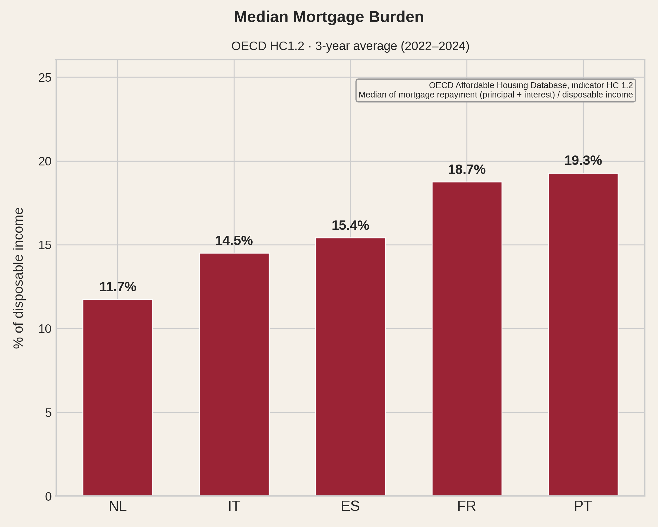
As a consistency check, we turn to an official source. In the opening section we saw that Eurostat's housing cost burden indicator excludes mortgage principal repayment, making cross-country comparison misleading. The OECD Affordable Housing Database, however, publishes a closely related indicator - the median mortgage burden as a share of disposable income - that includes principal repayment, without mixing in energy, maintenance, or insurance costs. This indicator is not granular - it irons out regional differences, as every national indicator does - and it measures something conceptually different from what we built: rather than estimating potential strain from simulated loans or simple effort ratios, it captures actual burden from self-reported mortgage payments in EU-SILC.
Because actual mortgage payments are sensitive to ECB key interest rates - and a large share of loans in these countries carries variable rates - we use a three-year average (2022-2024) to smooth year-to-year volatility.
The ranking is the same. Portugal carries the heaviest mortgage burden, followed by France, Spain, Italy, and the Netherlands - the order produced by our regional effort metric in Part four. Two indicators built from different data, at different scales, with different methodologies, point in the same direction.
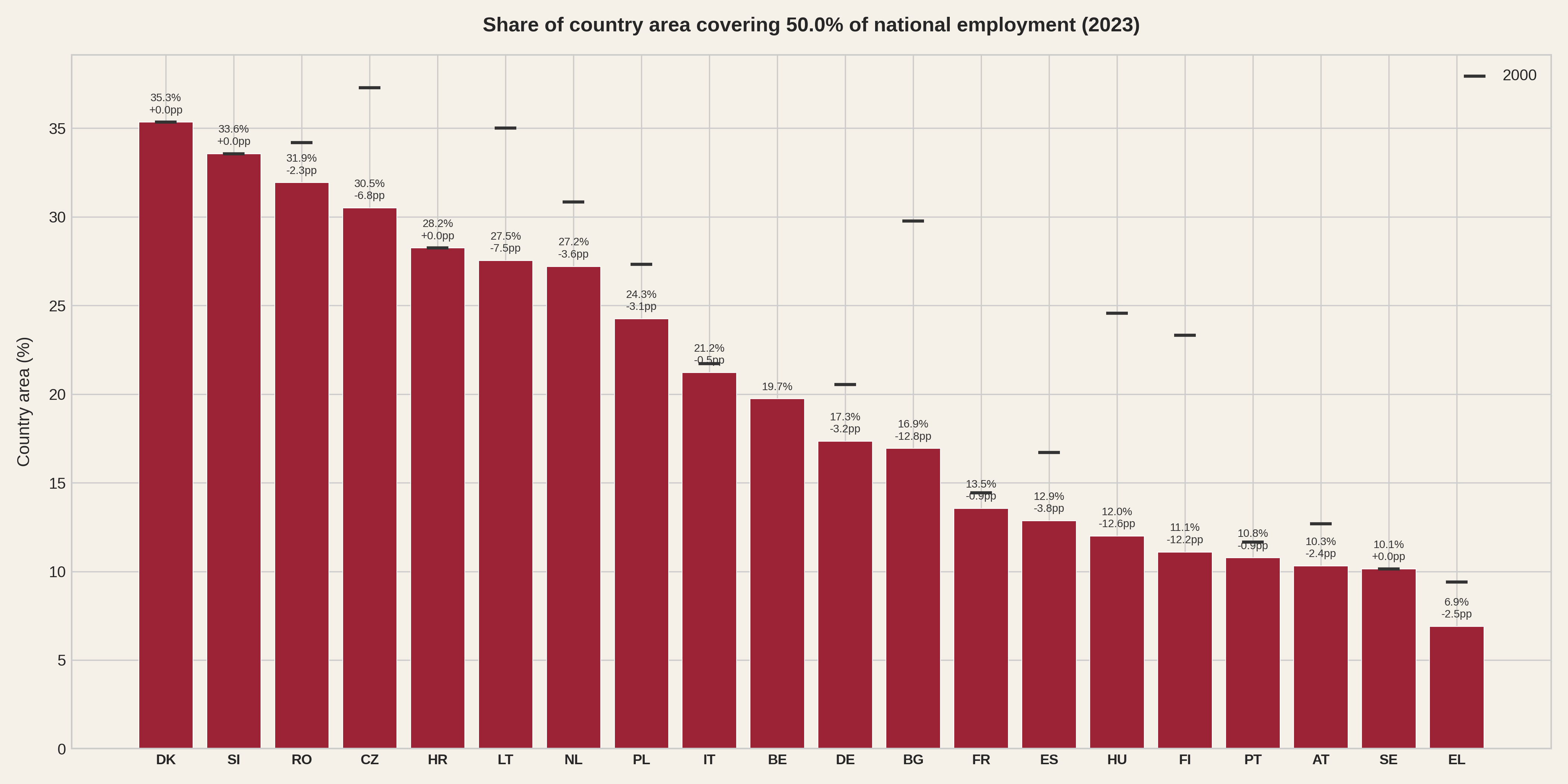
How concentrated is employment today? In Portugal, half of all jobs sit on just 11% of the country's land area. Spain packs them into 13%, France into 14%. And since 2000, the picture got worse for almost every country. In Spain the area needed to cover half of employment shrank by 3.8 percentage points, in the Netherlands by 3.6. Across the EU, the trend is even starker: Bulgaria lost 13 points, Hungary and Finland 12.
How much of each country's territory hosts half its jobs? Black marks show the same metric in 2000. Belgium has no mark because Eurostat employment data for Belgian NUTS-3 regions only starts in 2003.
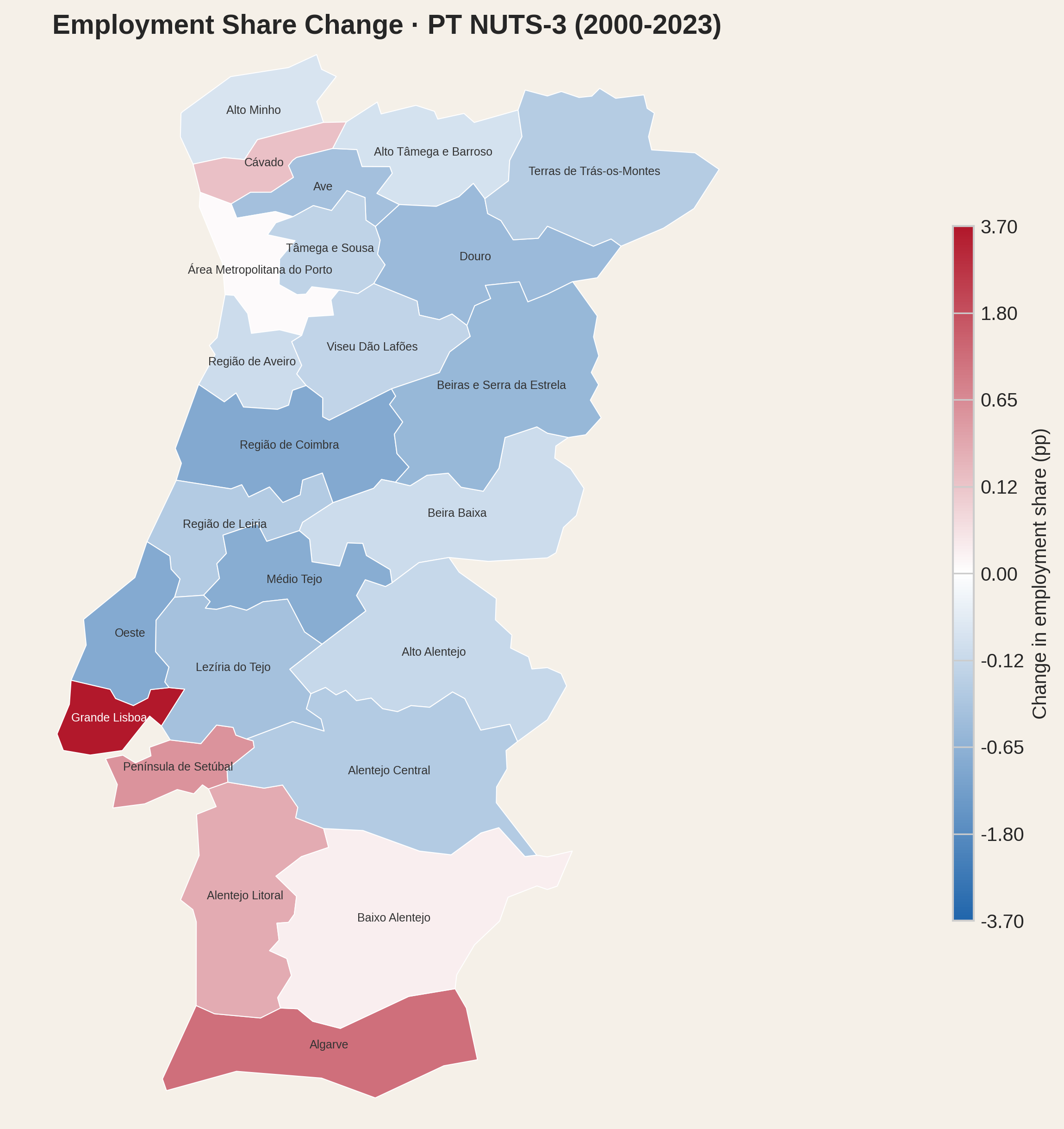
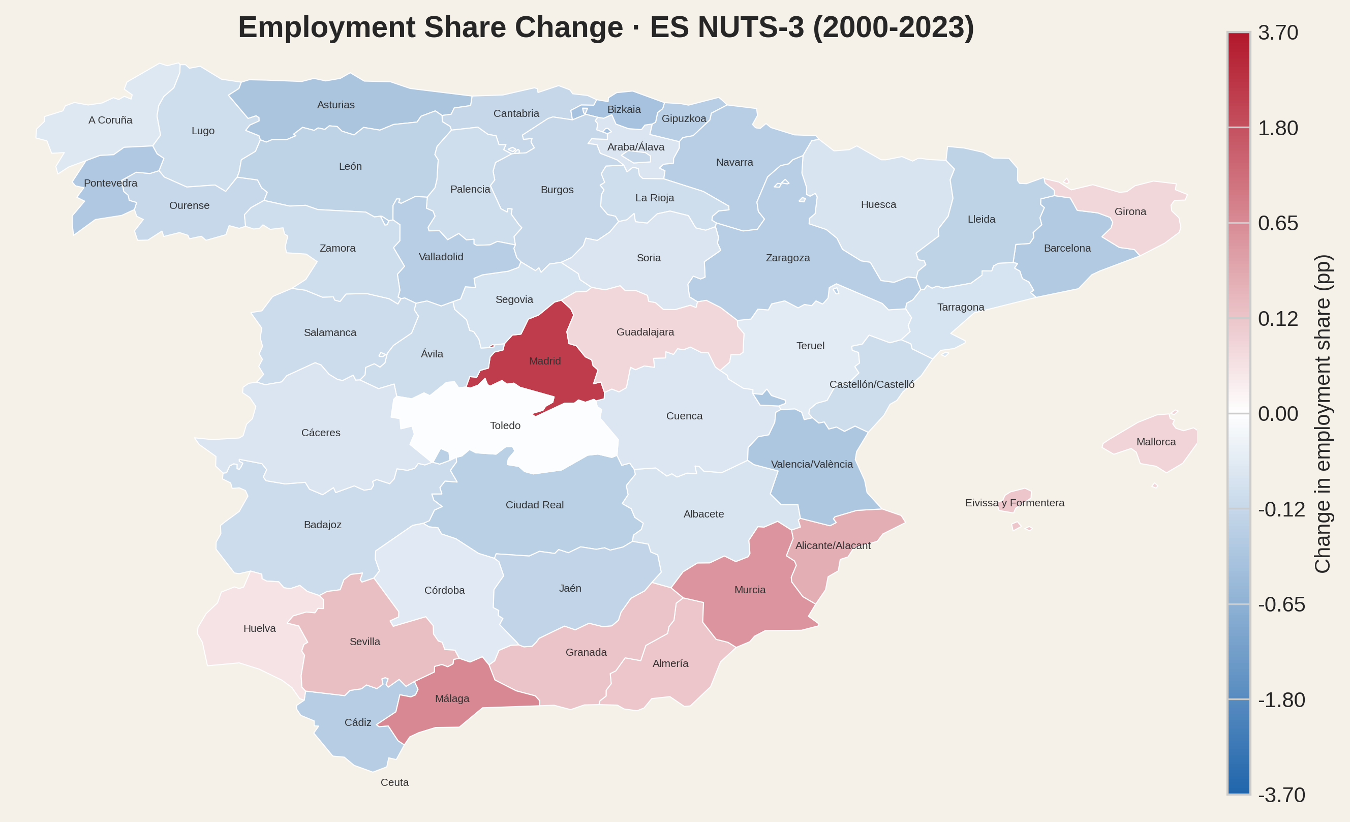
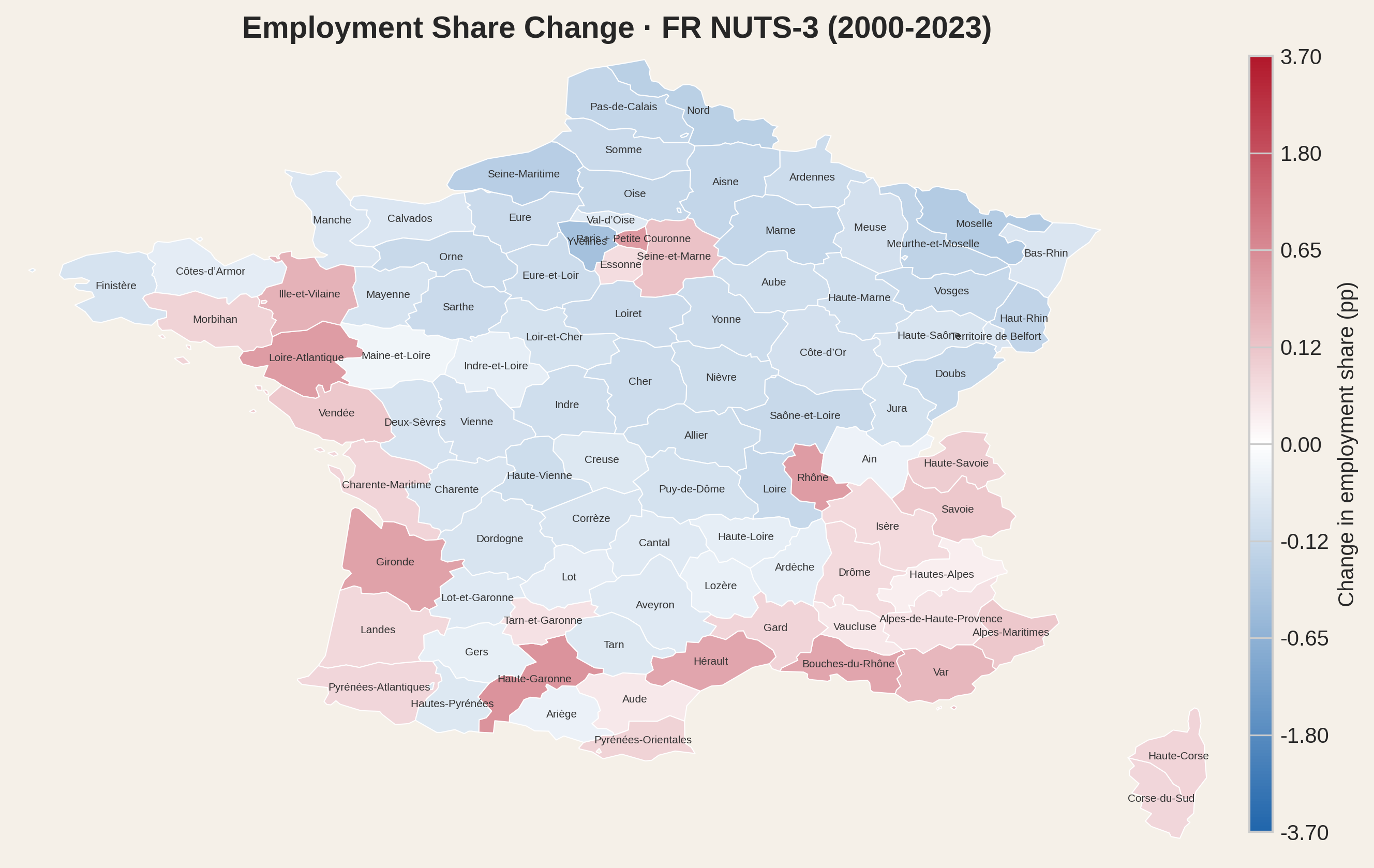
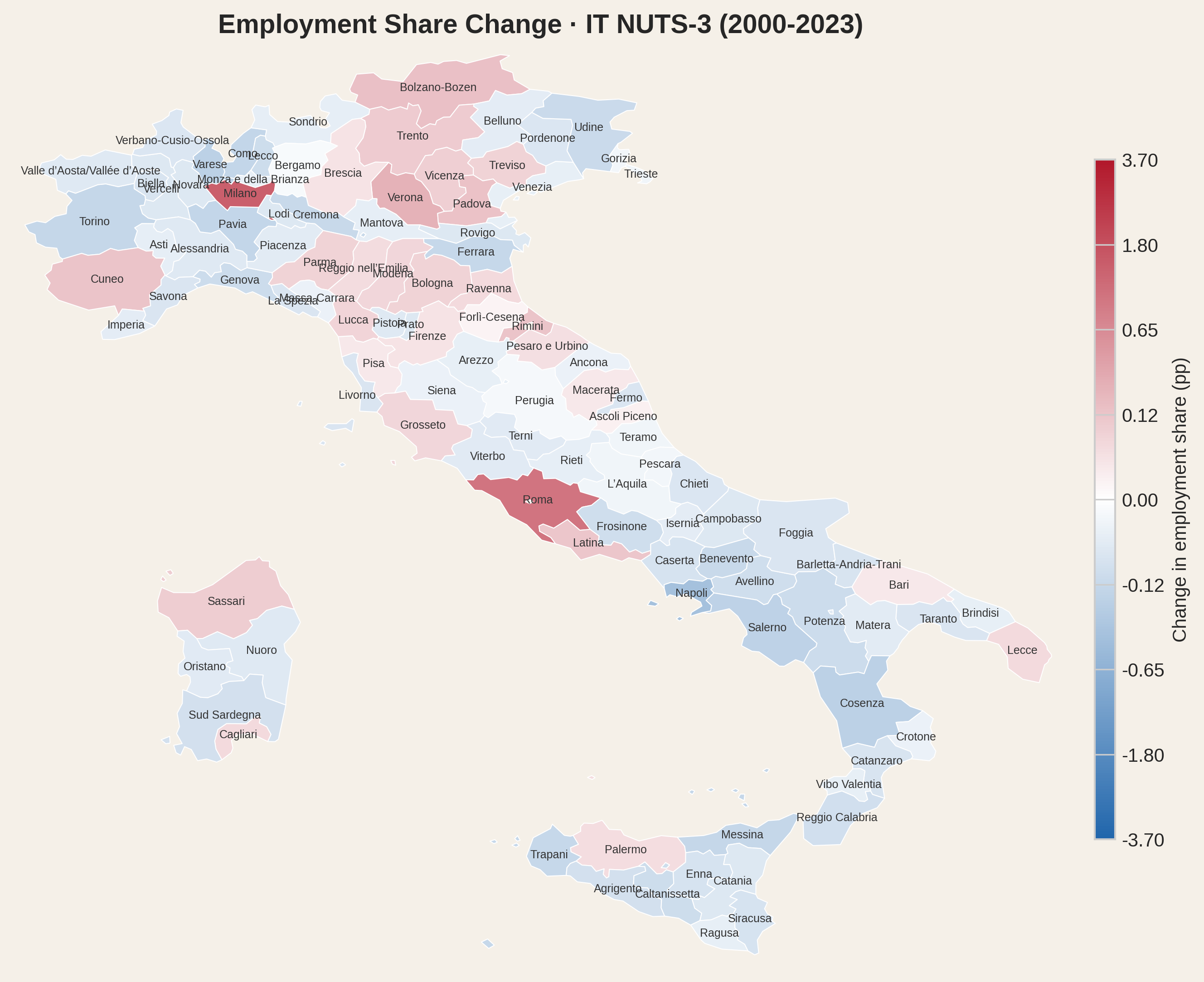
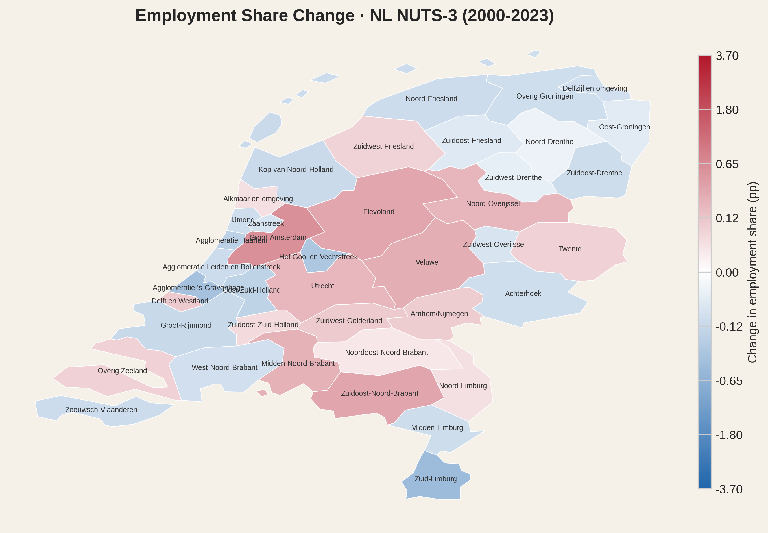
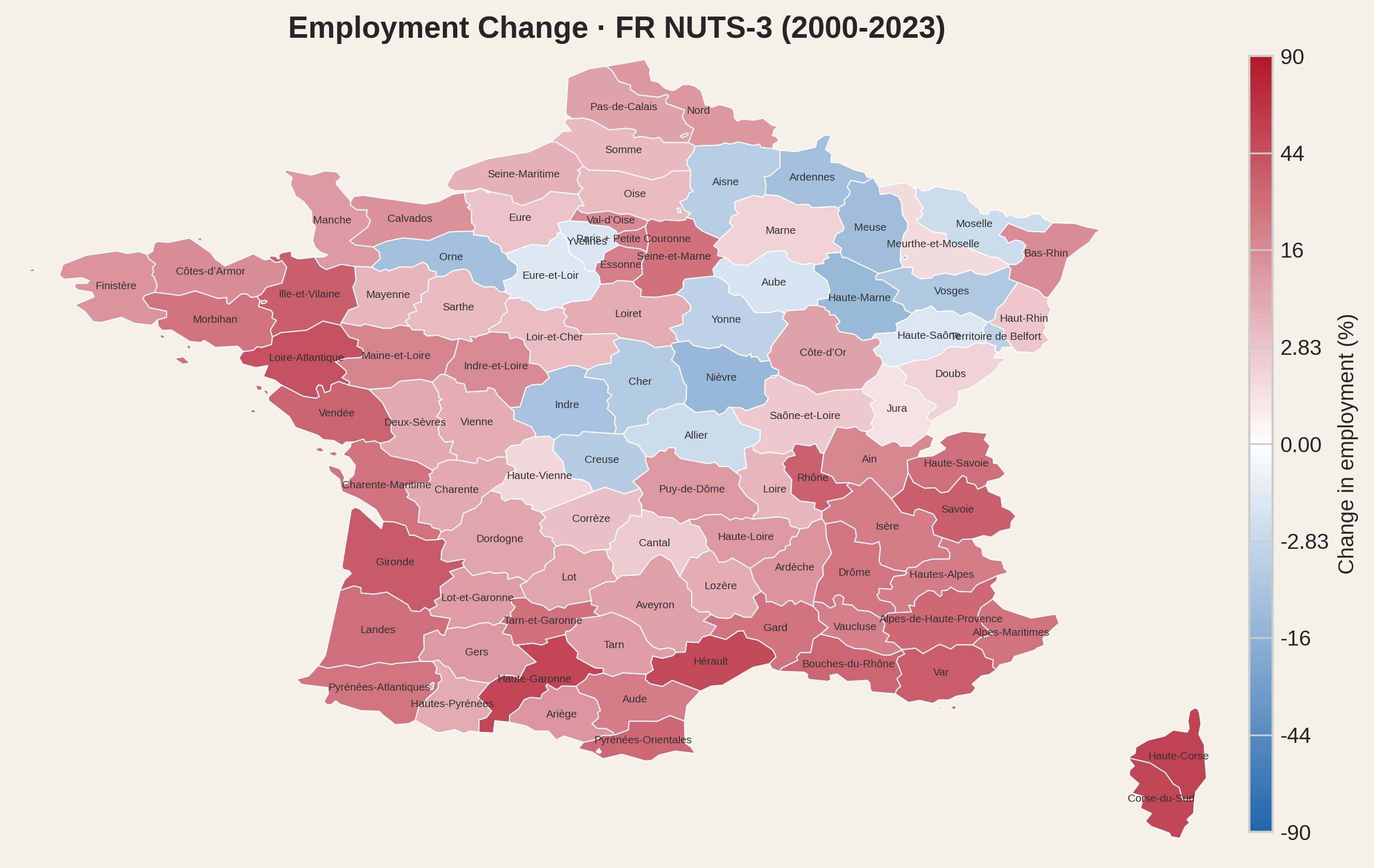
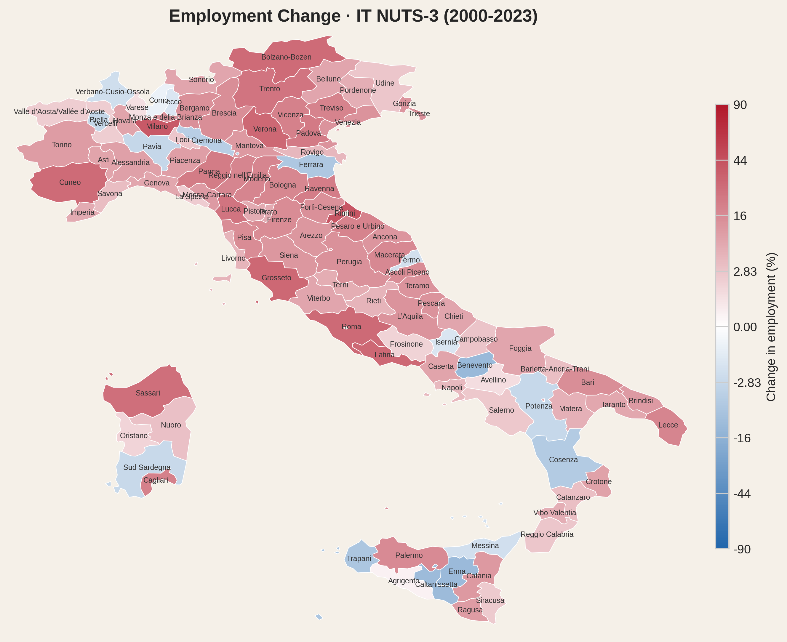
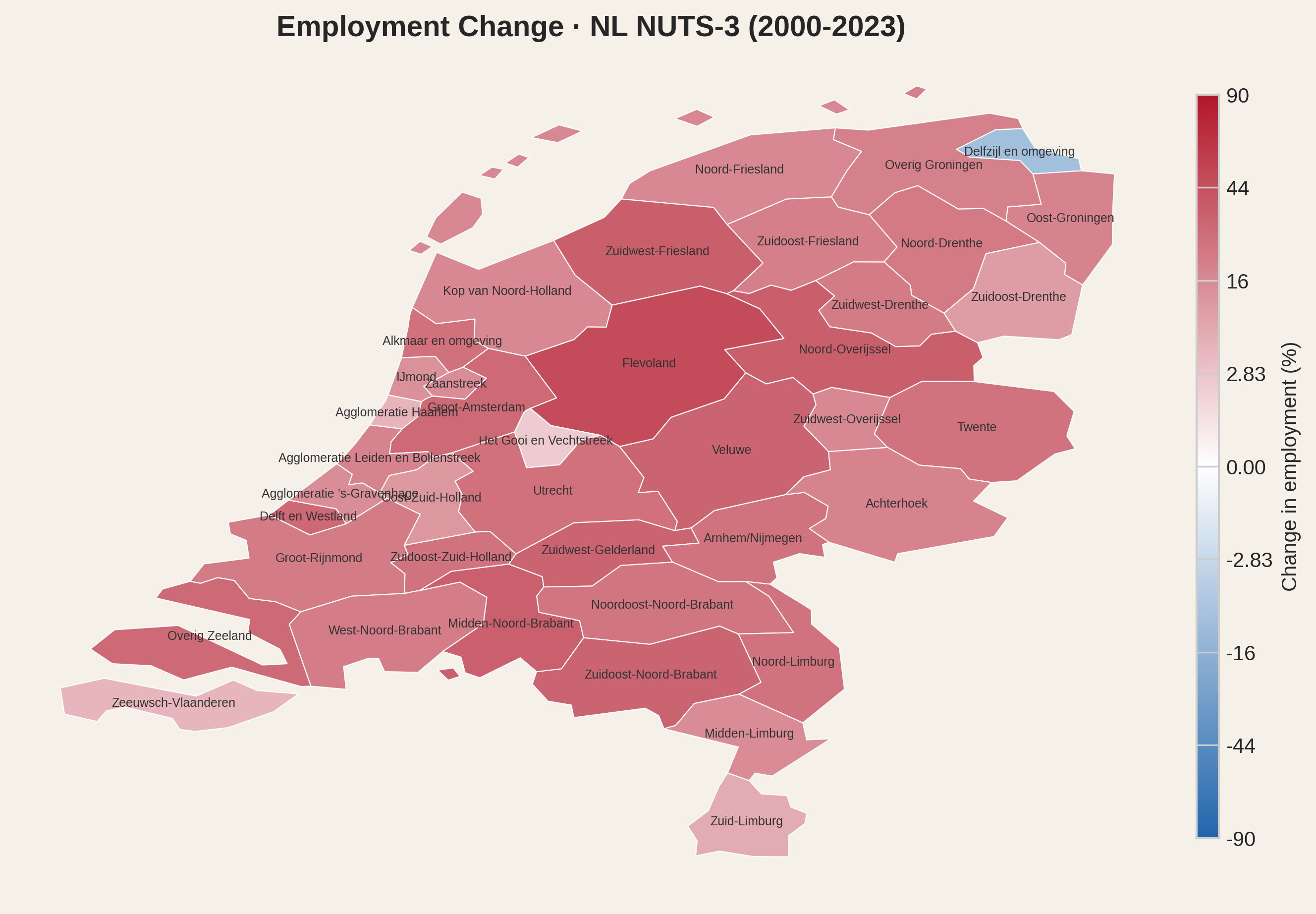
Country-level numbers, however, flatten the story. Mapping the change in each region's share of national employment between 2000 and 2023 reveals which regions gained importance and which regions lost.
Portugal
Spain
France
Italy
Netherlands
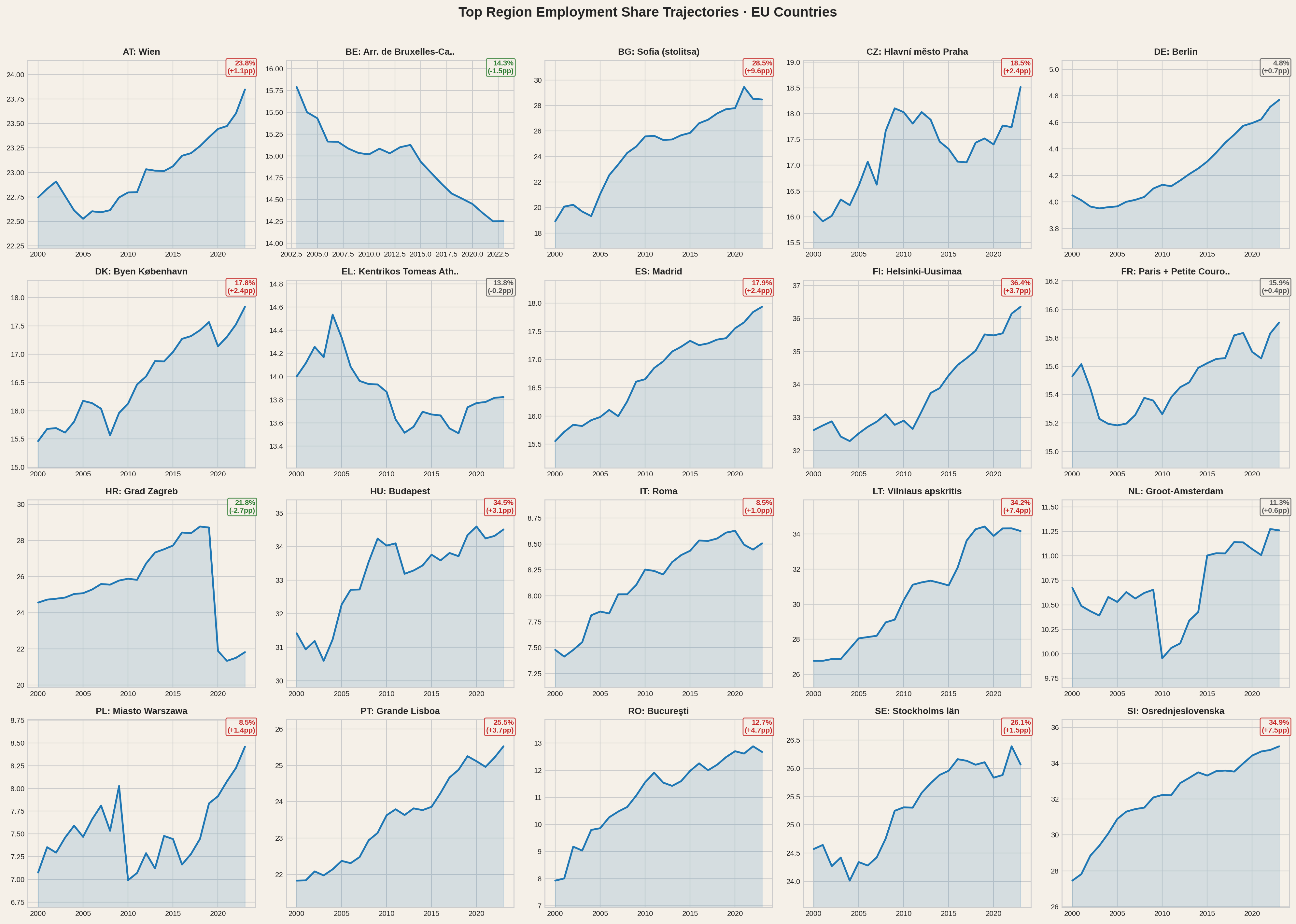
The pattern is consistent: capital regions and their satellites pull in red, while the interior fades blue. Tracking the top employment region in each EU country over two decades confirms the trend is not slowing down.
The capital region's share of national employment over time. In most countries, concentration has been stable or rising - decentralisation remains the exception, not the trend.
Net change in the capital region's employment share since 2000. Positive means the capital grew its dominance; negative means some dispersal occurred.
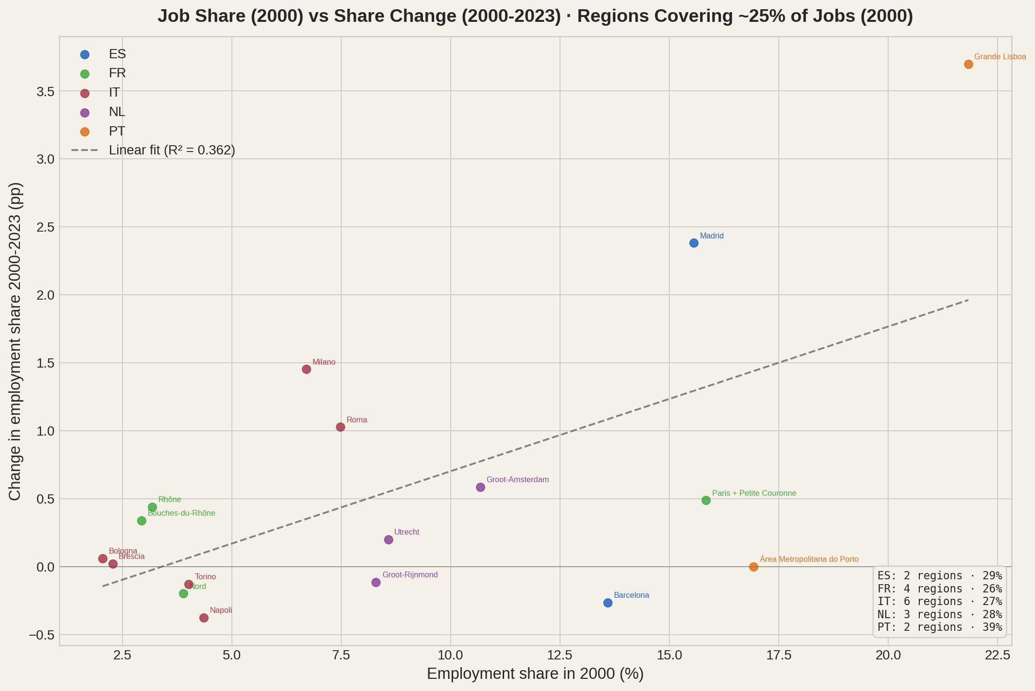
We have seen that most countries in Europe increased their employment concentration levels. The maps showed the geography and magnitude of that evolution, region by region. The top-region charts confirmed that capital regions follow this trend. One verification remains: did regions that already held a large share of jobs in year 2000 generally gain more employment share? Let's investigate for the five countries under study.
For each country, only the regions that together cover ~25% of national employment in 2000 are shown. All five capital regions gained share.
Every capital region gained employment share - from Paris (+0.5 pp) to Lisbon (+3.7 pp). Among the twelve non-capital regions in this selection, the story is not simple: five gained share (led by Milano at +1.5 pp), five lost (led by Napoli at -0.4 pp), and two were essentially flat (Porto and Brescia). This sample size is, by construction, small, so generalizations are difficult. Increasing the sample by setting the percentage threshold to ~50% would show more regions but does not uncover a clear pattern. In fact, we find that the dynamics of small job share changes on top of small initial job shares to be complicated and highly country dependent. The concentration story is not about all large regions increasing their relative importance - it is about capitals pulling away and runners-up working their ways, with mixed outcomes.
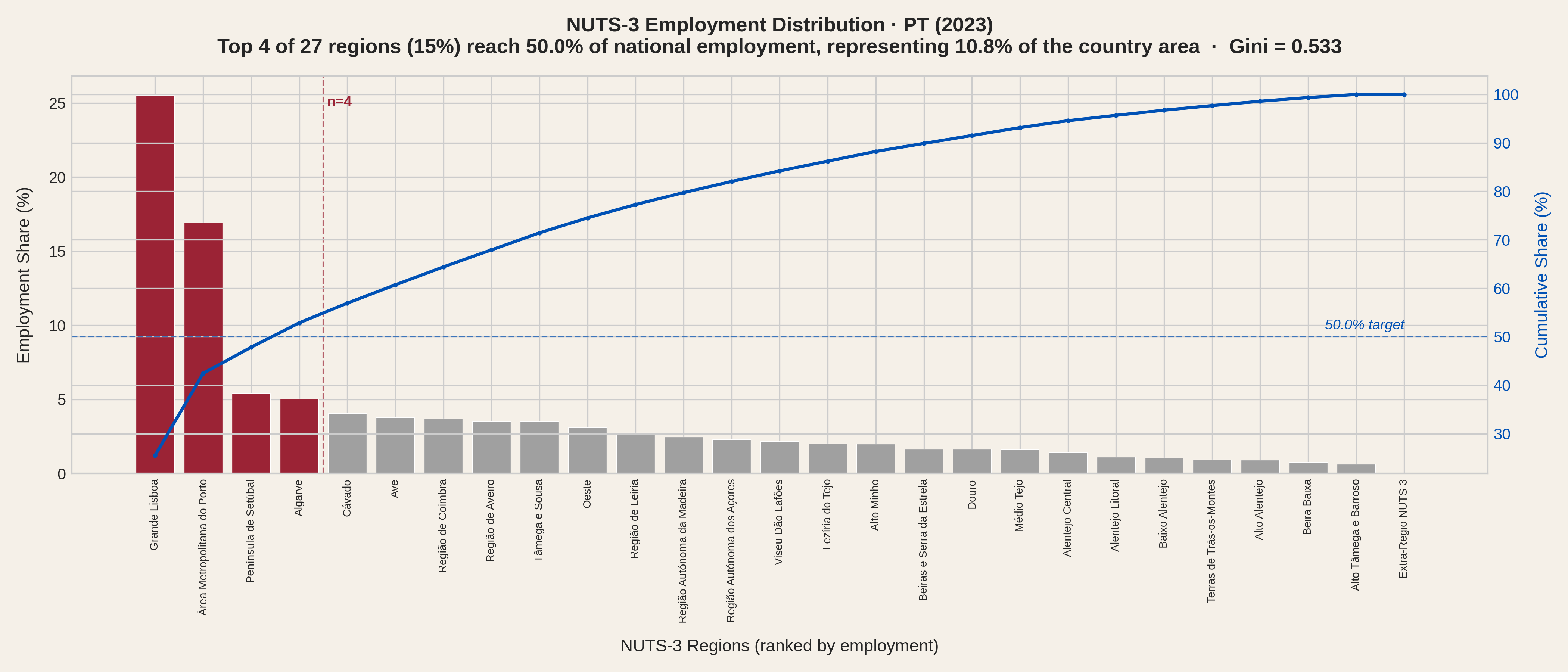
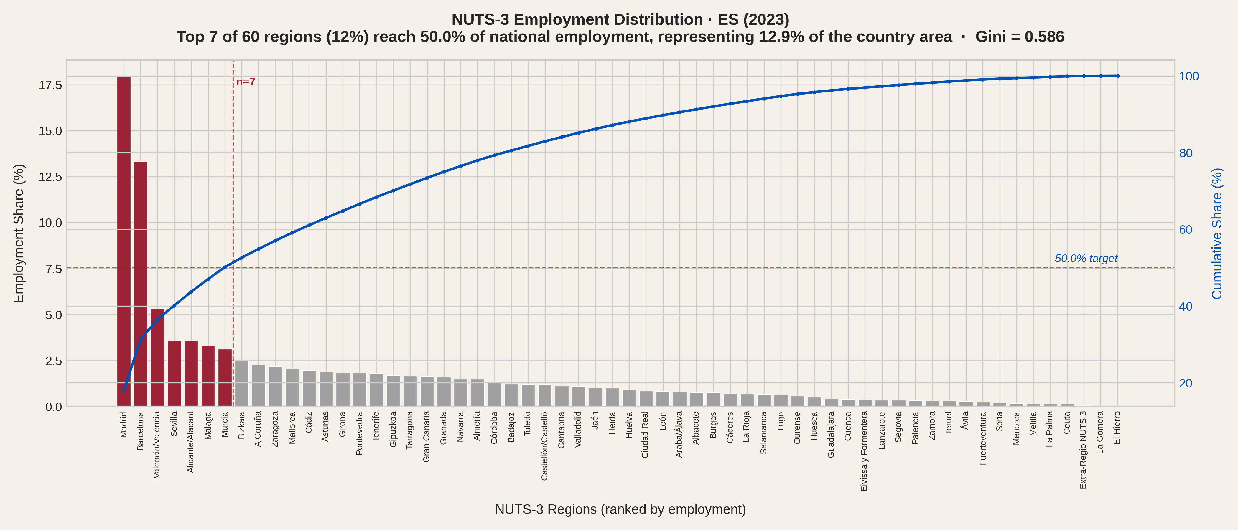
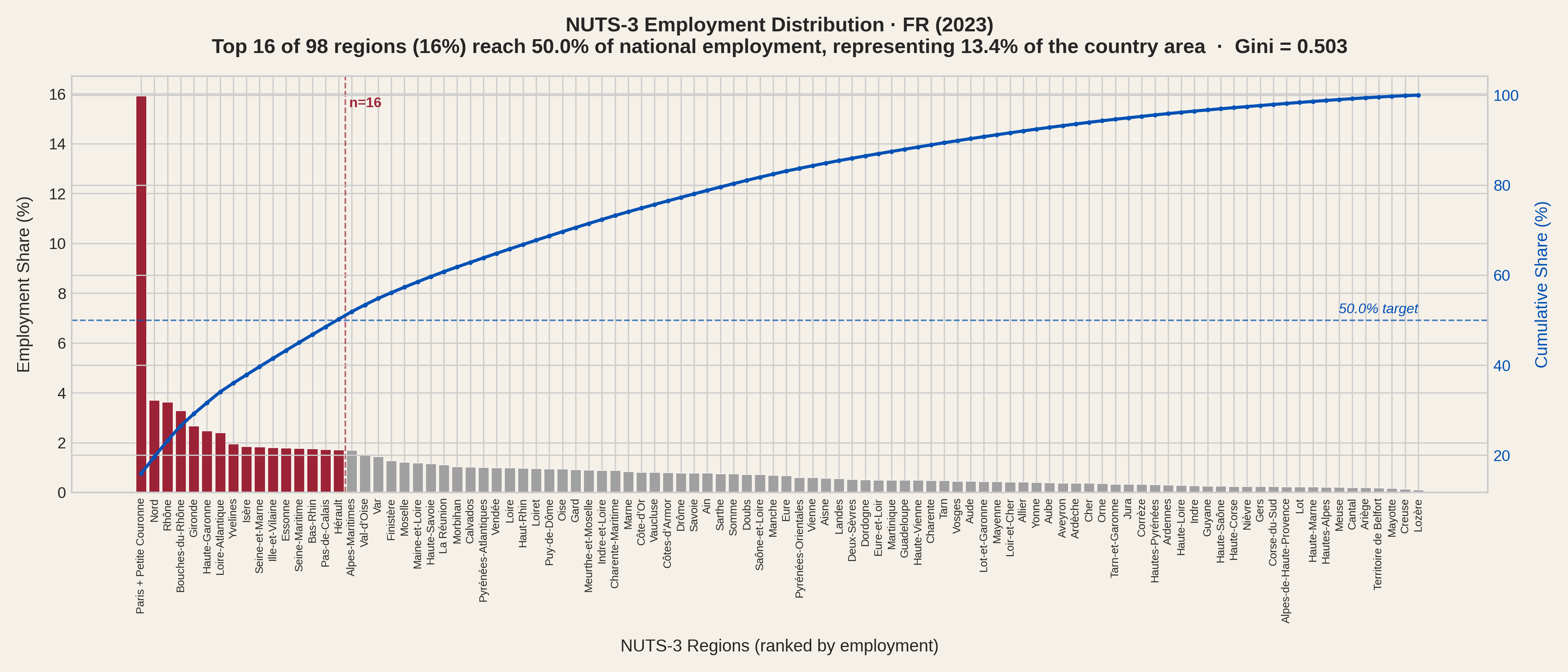
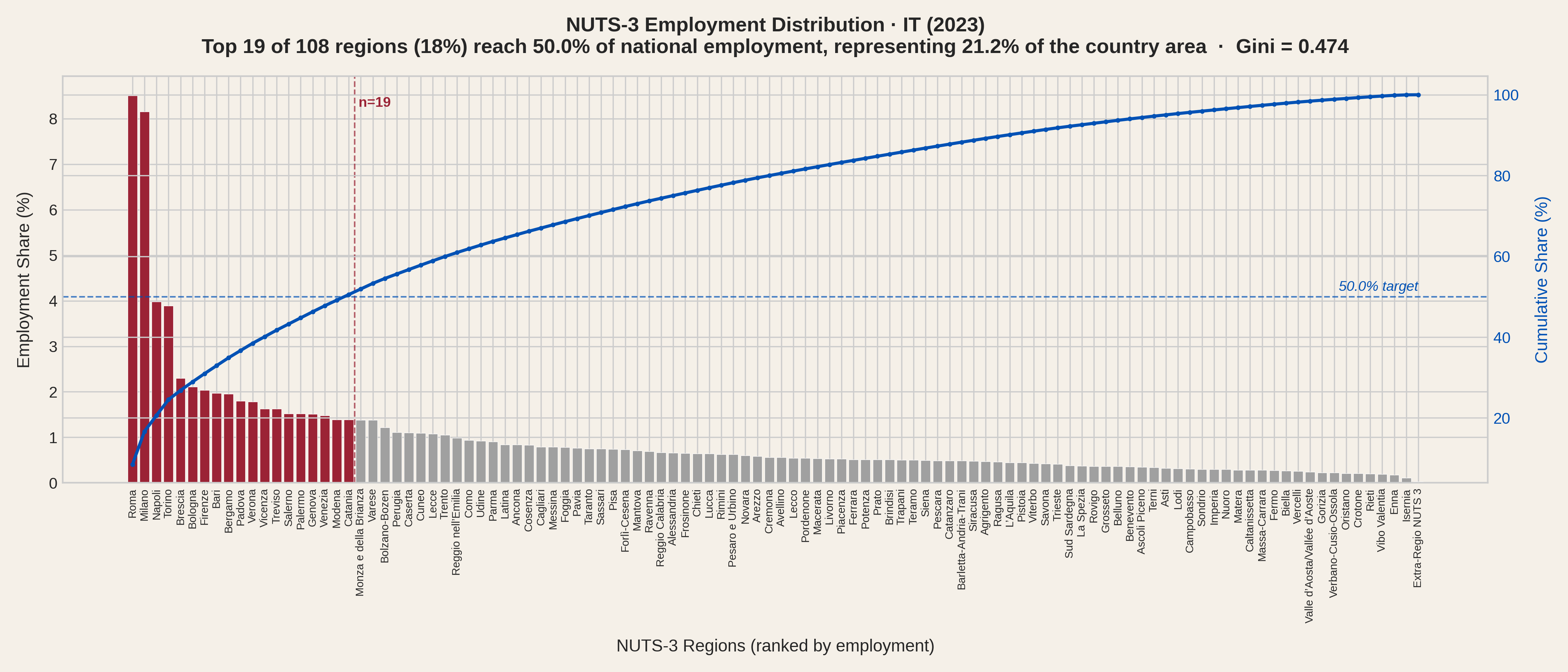
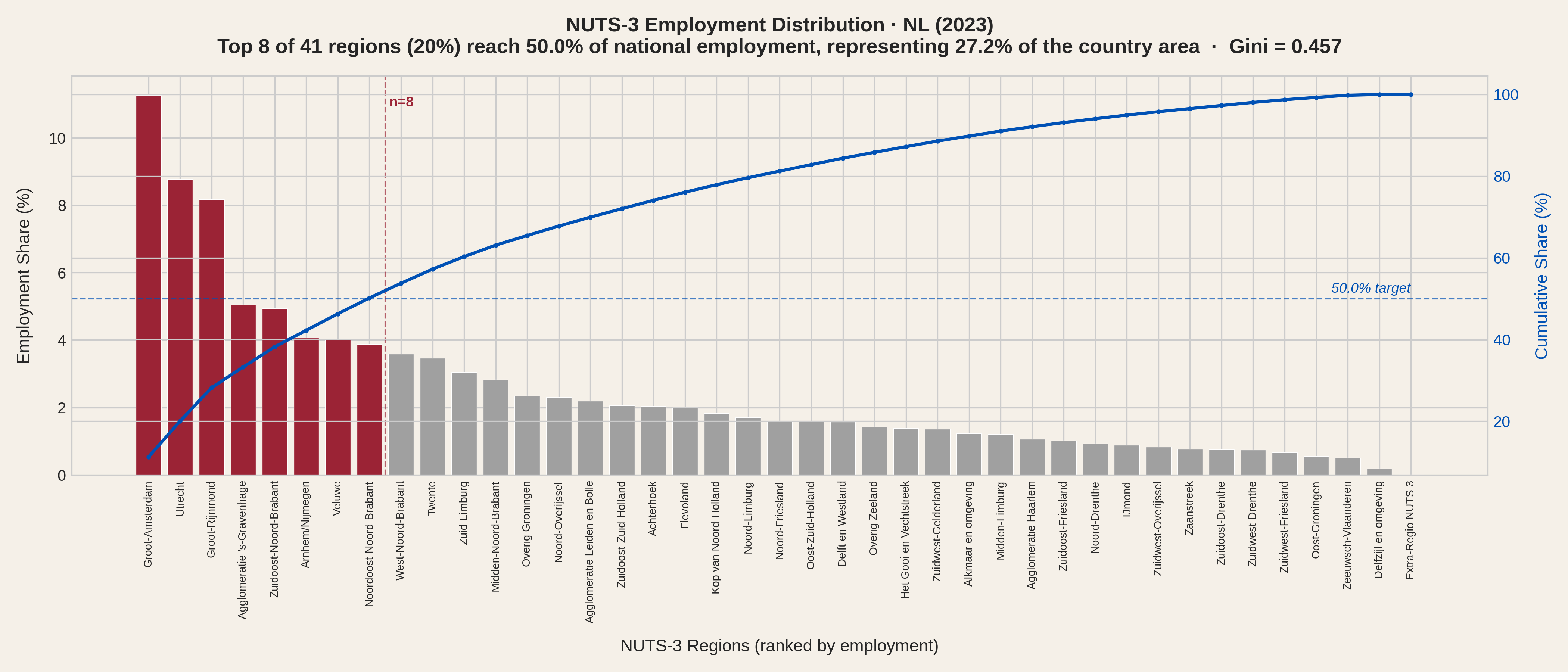
What is the net result? The distribution plots below rank each country's NUTS-3 regions by employment and show how many it takes to reach 50% of the national total. Portugal needs just 4 regions, Spain 7, the Netherlands 8, France 16 and Italy 19.
Portugal - 4 regions cover 50% of national employment.
Spain - 7 regions cover 50%.
France - 16 regions needed, with Paris + Petite Couronne holding 15.9%.
Italy - 19 regions, reflecting its polycentric structure.
Netherlands - 8 regions, with a smoother tail than Portugal or Spain.
These plots illustrate well the significant concentration, especially in Portugal, Spain and France. Half of the jobs are in 11% - 14% of the area, for these 3 countries. Italy and The Netherlands show less extreme results, which is compatible with the overall better affordability found for those countries.
The Gini coefficient, a standard measure of inequality that can also be applied to the employment distribution across the regions of a country, confirms the picture: Spain leads at 0.59, followed by Portugal (0.53) and France (0.50), while Italy (0.47) and the Netherlands (0.46) are more evenly spread. A Gini of zero would mean every region has the same number of jobs; a value approaching one would mean all jobs are in a single region.
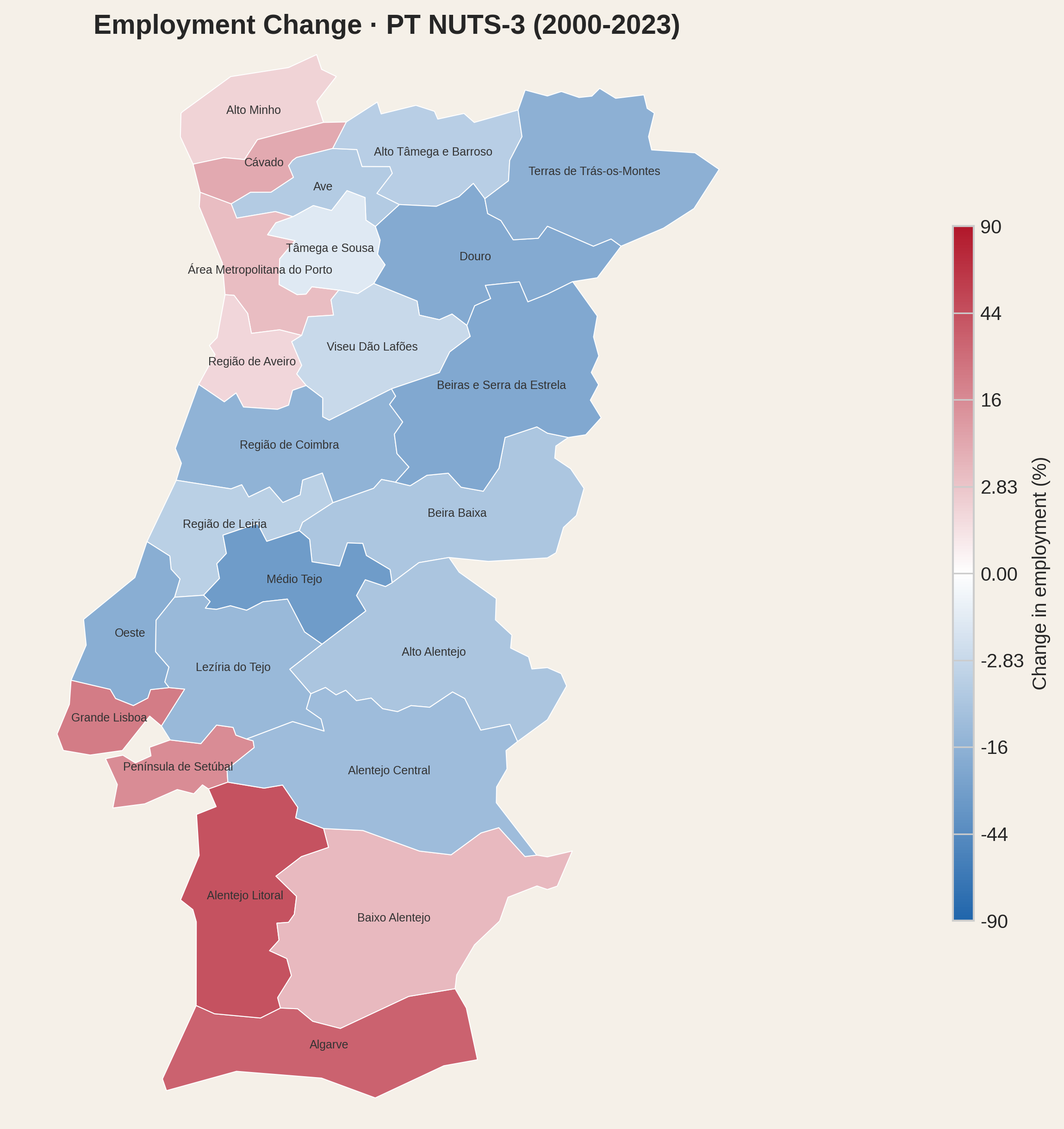
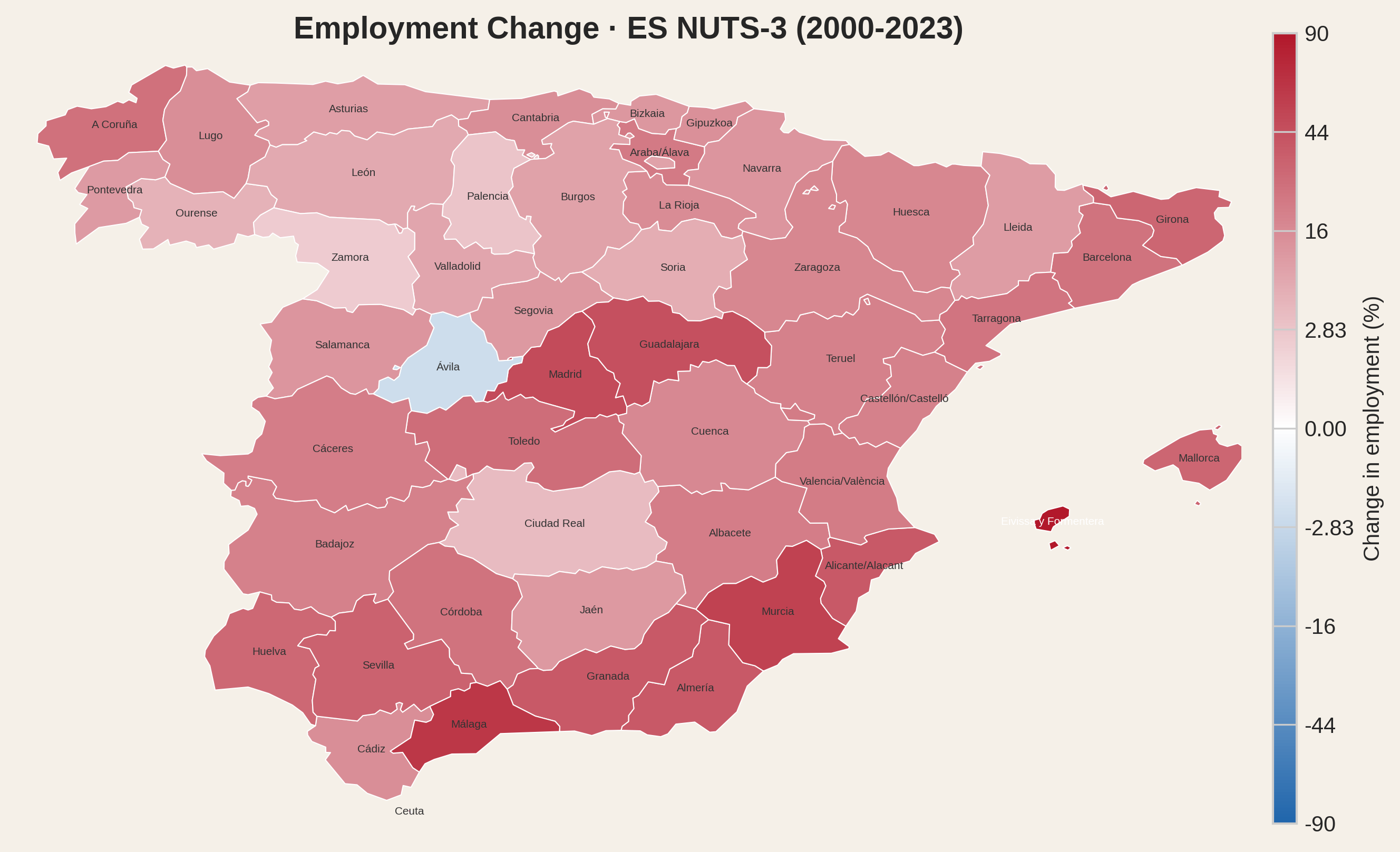
At this point, we should note that the share statistics are a zero-sum view - we have seen which regions gained relative importance from 2000 to 2023 and we have seen the resulting employment distribution for 2023. But what happened to employment in absolute terms? That last insight will be provided by the following maps.
Portugal
Spain
France
Italy
Netherlands
The employment variation numbers highlight differences between countries. In Spain, nearly every region gained jobs - but the share map shows Madrid ate a significant slice, reinforcing its already dominant share. In Portugal, the interior didn't just fall behind relatively: Douro lost a fifth of its workforce and Trás-os-Montes lost a sixth. Italy and the Netherlands had absolute gains in almost all regions. France shows gains in most regions with losses in a smaller, but significant, number. But there is something in common: every capital region had double-digit growth. Absolute employment gains for capital regions are in the range of 21% (Paris + Petite Couronne) to 48% (Madrid). For the capital regions of these five countries, increased employment share came hand in hand with double-digit growth of employment density, generating outstanding pressure in the housing market.
Two findings stand out.
First, housing purchase effort is structurally correlated with employment density across all five countries under study. The simplest explanation is causal: when more workers compete for the same land, prices rise relative to wages. Second, that pressure has been intensifying. Since 2000, every capital region recorded double-digit employment growth - not as an isolated boom but as part of a broader trend in which the share of national employment concentrated around capitals has increased. More jobs, more people, same land - the mechanism is self-reinforcing.
The chronically lagging supply is not attributable to a single problem. Many have been publicly mentioned: lack of space, permit bottlenecks, manpower scarcity, expensive credit, zoning laws, political obstacles. Whatever mix affects one region is different from the mix of another, even the effect being the same. Some argue for more houses; others argue for price controls. It is hard to imagine that the affordability problem in dense regions will be solved using either simplistic approach. And the more concentration increases the more the solution is dependent on a few regional administrative structures - hostage to whatever logistical issues or political biases affect the dominating regions. As that happens, people will, most likely, remain strained - and productivity, fertility and well-being will suffer. Density and concentration are rarely part of that conversation, which is what motivated this study. Could decentralisation be part of the solution?
The COVID-era experiment with remote work briefly suggested a different future. Workers discovered they could live in affordable regions and earn urban salaries. Housing pressure on dense areas eased, if only slightly. Secondary cities saw new demand. In 2020, the question was suddenly legitimate: do we all need to be on 11% of the land to do our jobs?
That window is closing. Return-to-office mandates, the gravitational pull of face-to-face networks, and policy inertia are reassembling the old pattern. The structural incentives that concentrate employment have not changed: agglomeration economies, headquarters bias, infrastructure investment tilted toward capitals.
Return-to-office mandates, one after another, are not just HR policies. They are housing policies. Every RTO memo that says "three office days in Lisbon / Madrid / Paris" is also a memo that says "and therefore 24/23/37 years of mortgage for a 50 m²". We re-concentrated on purpose, after seeing what de-concentration looked like.
Every fiscal incentive that only rewards a headquarters in the capital, every high-speed line that only connects capitals, every new university campus that opens inside the same 11% - is a peanut in the corner. Employment concentration is the elephant in the house - the structural force that no amount of tinkering with mortgage rates, construction permits, or tourist regulations will fully overcome. The elephant will not move while we keep feeding the corner.
All data is from 2023 except where noted, using the NUTS 2024 classification and boundaries. Eurostat employment and tourism series for 2023 are already published in NUTS 2024 codes for the five countries in this study. French wages use 2022 (latest available). Regions using Eurostat NUTS-2 fallback wages are flagged and excluded from regression fits. Full data and source code are available in the project repository.
All source data is publicly available. Eurostat datasets cover the full EU; national sources cover NUTS-3 regions within each country. The Local copy column links to our downloaded snapshot used for this analysis.
| Dataset | Source | Coverage | Local copy |
|---|---|---|---|
| Employment (all countries) | Eurostat - nama_10r_3empers | NUTS-3, employed persons (thousands) | csv |
| Land area (all countries) | Eurostat - reg_area3 | NUTS-3, km² | csv |
| Tourism nights (all countries) | Eurostat - tour_occ_nin2 | NUTS-3 (NUTS-2 in some countries) | csv |
| Share of housing costs in disposable household income (all countries) | Eurostat - ilc_mded01 (EU-SILC) | Country level, total households | csv |
| Financial burden of housing cost (all countries) | Eurostat - ilc_mded04 (EU-SILC) | Country level, total households | csv |
| Housing costs over income, HC 1.2 (all countries) | OECD Affordable Housing Database | Country level, median mortgage and rent burden | xlsx |
| NUTS-3 boundaries (all countries) | Eurostat - GISCO 2024, 1:10M | GeoJSON polygons | geojson |
| Housing prices (Portugal) | INE - indicator 0012235 | NUTS-3, median transaction price per m² | csv |
| Wages (Portugal) | MTSS - Quadros de Pessoal | NUTS-3, mean monthly earnings (ganho) × 14 | csv |
| Housing prices (Spain) | Colegio de Registradores - Portal Estadístico | Province, mean transaction price per m² | csv |
| Wages (Spain) | AEAT - Mercado de Trabajo (IRPF) | Province, mean annual salary | csv |
| Housing prices (France) | DGFIP - Demandes de Valeurs Foncières (DVF) | Département, median transaction price per m² | csv |
| Wages (France) | INSEE - DADS/DSN T401b | Département, gross annual salary EQTP (2022) | csv |
| Housing prices (Italy) | Agenzia delle Entrate - OMI quotazioni | Province, appraised market values per m² | csv |
| Wages (Italy) | INPS - Osservatorio lavoratori dipendenti | Province, mean gross annual pay | csv |
| Housing prices (Netherlands) | CBS - StatLine (Bestaande koopwoningen) | COROP, mean transaction price per m² | csv |
| Wages (Netherlands) | CBS - StatLine (Regionale rekeningen) | COROP, compensation per employee (÷ 1.27) | csv |
The following datasets are produced by the analysis scripts and underpin the charts in this story. Each file can be downloaded for independent verification.
| File | Description | Section |
|---|---|---|
| others_housing_cost_burden_2023.csv | Share of housing costs in disposable household income, by country (Eurostat EU-SILC) | Part 1 |
| others_housing_burden_subjective_2023.csv | Subjective housing burden by country — heavy, some, none (Eurostat EU-SILC) | Part 1 |
| others_oecd_mortgage_burden_2022_2024.csv | Median mortgage burden by country, 3-year average (OECD HC1.2) | Part 8 |
| dvp_PT_ES_FR_NL_IT_effort_2023.csv | Region-level density, prices, wages, effort and tourism for NUTS-3 regions | Parts 3–8 |
| dvp_PT_ES_FR_NL_IT_summary_2023.csv | Country-level employment-weighted mean effort | Part 4 |
| dvp_PT_ES_FR_NL_IT_multivar_fit_2023.csv | Multivariate fit: predicted vs actual effort per region | Part 5 |
| dvp_PT_ES_FR_NL_IT_extra_fit_evidence_2023.csv | R² for density-only and tourism-only fits per country | Part 5 |
| concentration_share_delta_2000_2023.csv | Employment and employment share per NUTS-3 region, years 2000 and 2023 | Part 9 |
| concentration_top_region_timeseries.csv | Top-region employment share trajectories, EU countries | Part 9 |
| concentration_share_scatter_2000_2023_target25pct.csv | Share scatter: regions covering ~25% of national employment | Part 9 |
This analysis requires three datasets at NUTS-3 level for every country: housing prices per m², wages, and employment. No single European source publishes all three. Each country must be assembled from national statistical offices, tax authorities and property registries - each with its own methodology, coverage and access conditions. Portugal, Spain, France, Italy and the Netherlands are the five where the necessary data could be obtained at comparable quality. Germany was investigated but its regional price data (AK OGA) is published only as binned ranges, not as values usable in regression. Denmark's wages are available only at NUTS-2, too coarse for this analysis. Other countries face similar gaps. Expanding coverage is a matter of data access, not methodology.
2023 is the most recent year for which all five countries have both housing prices and wages at NUTS-3 level. France is the binding constraint - INSEE publishes regional wages with a one-year lag, so 2022 wages are the latest available and are used as a proxy for 2023. Portugal's transaction price series (INE 0012235) starts in Q4 2019, making anything before 2020 unavailable at comparable quality. Italy's INPS wage data begins in 2019. Tourism data from Eurostat (tour_occ_nin3) switched to NUTS 2024 codes in 2023, making that the only year where tourism intensity can be matched to the current regional boundaries without manual code reconciliation. The housing cost burden chart uses the same 2023 reference year as the rest of the analysis.
Cross-country comparisons should be read with care. The wage concept differs: Portugal (MTSS Quadros de Pessoal) and Italy (INPS) cover private-sector employees only, while Spain (AEAT) and France (INSEE DADS) include all sectors. The Netherlands (CBS) reports compensation of employees - gross salary plus employer social contributions - which is corrected by dividing by 1.27 to approximate gross salary. Within each country all regions use the same concept, so regional rankings are unaffected.
Housing prices also differ in concept: Portugal and France use median transaction prices from notarial records; Spain and the Netherlands use mean transaction prices; Italy uses expert-appraised market value ranges (OMI quotations), not actual transactions. Mean prices are typically 5-15% higher than medians due to luxury outliers. The Italian figures are methodologically closer to valuations than to recorded sales.
There are also differences between national definitions of dwelling floor area. These include the treatment of common areas in apartment buildings, balconies and terraces, as well as other spaces such as cellars, attics and storage rooms. Consequently, the reported price per square metre is not based on a perfectly harmonised measure of floor area across countries.
Per-country scatter plots and regressions are reliable. The combined multi-country plots are useful for seeing overall patterns but should not be read as precise cross-country rankings.
Visitor nights per worker is a NUTS-3 average. In a capital region, tourists cluster near the city centre while the workforce spreads across the whole metropolitan area, so the metric undercounts tourism pressure where it is most intense and dilutes it across suburbs where it barely exists. In regions like Algarve or Corsica, where tourism is the defining activity across the territory, visitors are more distributed and this average is far more representative of reality. Naturally, when comparing regions, this nuance can only be evaluated qualitatively, because NUTS-3 is the finest granularity we have data for.
NUTS-3 boundaries follow administrative divisions, not a standard grid. Paris (FR101) is 103 km² - just the city proper. Madrid (ES300) is 7,972 km² - the entire province, including sparsely populated countryside. Grande Lisboa sits between at 1,322 km²; Rome covers 5,280 km². This matters most for employment density: Paris registers 21,700 jobs per km² while Madrid shows 484 - a 45-fold difference that is largely a boundary artefact, not a real difference in urban intensity.
Housing effort (price ÷ wage) is more robust, since both numerator and denominator are measured at the same geographic scale and area does not enter the calculation. However, large regions like Madrid average high-effort urban cores with low-effort rural fringes, which understates peak affordability pressure. Paris, by contrast, captures almost exclusively the dense, expensive centre - which is why its effort figure looks extreme even by capital-city standards. The adjacent Petite Couronne départements (Hauts-de-Seine, Seine-Saint-Denis, Val-de-Marne) have effort values of 1.1 to 1.3 - still elevated, but far below the 2.1 of Paris itself.
This is why in the cross-country scatter plots we merge Paris with its Petite Couronne into a single employment-weighted data point. The case for merging is straightforward. At 103 km², Paris is the smallest NUTS-3 region in our entire dataset - smaller than any region in Portugal, Spain, the Netherlands, or Italy. Even after merging with the three surrounding départements the combined area is just 753 km², still well below the median NUTS-3 area of 4,500 km² across our five countries. The four regions form a contiguous urban mass where housing markets are deeply intertwined: Paris prices would not sustain themselves without the millions of workers who commute from the Petite Couronne every day, and those same workers face housing costs inflated by their proximity to the centre. Treating Paris as an isolated data point overstates its density by an order of magnitude and places its effort on a mathematical cliff where small assumption changes produce wild swings. The merge does not hide the problem - Paris + Petite Couronne still ranks as the highest-priced and densest unit in our dataset - it simply brings the measurement closer to what the other capital regions already capture by default through their wider boundaries.
If anything, this intervention errs on the side of caution: the functional Paris labour market extends well beyond the Petite Couronne into the grande couronne and further, and a case could be made for merging a larger area still. We stop at four départements because they form the obvious contiguous core and because extending further would require judgement calls about where the commuter basin ends - a question that the NUTS classification was supposed to answer for us. None of this is a criticism of the NUTS-3 classification itself. EU regulation requires NUTS regions to follow existing administrative divisions within each member state, and for good reason: administrative units have the data-collection infrastructure, legal authority, and political legitimacy that purpose-built statistical areas would lack. France's départements date to the Revolution, designed so any citizen could reach the capital in a day on horseback - sensible for 18th-century governance, less so for 21st-century labour-market analysis.
Not every country maps NUTS-3 to a traditional administrative division. The Netherlands is the clearest exception: its COROP regions are non-administrative areas designed around commuting patterns. Portugal's Comunidades Intermunicipais are a hybrid - created to coordinate EU structural funding, they have no role in day-to-day governance, which remains with the individual municipalities. But France, Spain and Italy map NUTS-3 directly to long-established administrative divisions - départements, provincias, province - whose boundaries reflect centuries of political history. The Paris merge is our way of working with what we have: not redrawing the map, but acknowledging that one boundary was drawn too tightly for the question we are asking.
Per-country scatter plots and regressions are not affected - regions within the same country are drawn from the same administrative system and are reasonably comparable. The combined cross-country scatter plots use the Paris + Petite Couronne merge described above, which mitigates the most extreme size asymmetry. The x-axis (density) still mixes differently sized containers across countries, but no other region presents a distortion as severe as unmerged Paris.
The effort metric uses gross salary - the broadest wage concept consistently available at NUTS-3 level across all five countries. The exact source differs: Portugal uses mean monthly earnings from employer reports (MTSS Quadros de Pessoal, "ganho" × 14); Spain uses mean annual salary from tax returns (AEAT); France uses gross annual salary in full-time equivalents (INSEE DADS/DSN); the Netherlands uses total compensation of employees divided by headcount (CBS); and Italy uses mean gross pay from social security records (INPS).
These concepts are not perfectly harmonised. The Dutch figure includes employer social contributions, making it broader than the others. The Spanish figure comes from tax returns, which may undercount informal or irregular earnings. The Portuguese "ganho" includes overtime and regular bonuses beyond base pay.
We use gross rather than net salary because net wages are only published at NUTS-3 level in France. For the remaining countries, computing net salary would require modelling each country's tax and social security system - which varies by household composition, deductions, and (in Spain) by autonomous community. Disposable household income is available at NUTS-3 in four of the five countries, but not in Italy, and it includes non-work income (pensions, transfers, investment), which measures something different from what a worker earns. Gross salary, despite its imperfections, is the only metric that isolates worker income at the regional level across all five countries.
Outliers are detected in two steps. First, a log-linear model is fitted to all points (effort against ln(density)). The residuals of this initial fit are then tested using the interquartile range (IQR): points whose residual falls more than 1.5 × IQR below the first quartile or above the third quartile are flagged as outliers. The regression is then refitted without them. This is a standard non-parametric method that does not assume normally distributed residuals, and it is applied independently within each country so that cross-country differences in wage or price concepts do not influence which points are flagged.
Despite the comparability limitations described above, the single-variable fits are strong within each country. When countries are combined, the Portugal + Spain and Portugal + Spain + France subsets offer a good balance between sample size and methodological similarity: the Iberian pair shares a similar housing market structure and data tradition, while adding France extends the sample with a well-documented price source (notarial DVF data) and a comparable wage concept. In both combinations the role of the outliers identified in the individual Portuguese and Spanish fits is confirmed with higher statistical confidence thanks to the larger sample.
The two-variable model uses a logarithmic term for density and a linear term for tourism intensity. The logarithm captures the expectation that density's contribution to housing effort has diminishing returns: workers who pay for housing, whether through mortgages or rents that ultimately reflect purchase prices, are constrained by their wages and by credit rules. After the 2008 financial crisis, banking regulation tightened debt-to-income limits across Europe, not primarily to protect borrowers from high effort, but to protect the banking system from systemic risk. These constraints act as a ceiling: as density grows, effort cannot grow without bound. A logarithm approximates this saturating behaviour.
Tourism intensity, by contrast, enters linearly. The demand that tourism brings to a housing market can be inelastic to price: if a region reaches full accommodation capacity and prices rise, the visitor profile may shift to higher-paying segments rather than the volume declining. The supply of housing is locally rigid, but the pool of potential visitors is drawn from a global market whose purchasing power is large relative to any single region's stock, especially when that purchasing power is time-shared across the same property, as in short-term holiday rentals.
As an empirical check, we fitted the alternative model effort = a · ln(density) + b · ln(tourism) + c, replacing the linear tourism term with a logarithmic one. The R² was lower for four of five countries and for the pooled sample: the linear tourism term provides a better fit, consistent with the argument above.
Part one uses two Eurostat EU-SILC indicators. The first, ilc_mded01, reports total housing costs as a share of disposable household income. Housing costs are defined as rent (for tenants) or mortgage interest (for owners), utilities, structural insurance, mandatory services, maintenance, and housing-related taxes. Mortgage principal repayment is explicitly excluded on the grounds that it constitutes saving rather than expenditure. This means the indicator captures the interest component of a mortgage payment but not the principal component, systematically understating the cash-flow burden for homeowners with active mortgages.
The second indicator, ilc_mded04, is a subjective measure: households report whether housing costs represent a heavy burden, some burden, or no burden. For the five countries in this analysis, the subjective ranking (NL least burdened, ES/IT most burdened) contradicts the calculated one (NL most burdened, PT least). The divergence illustrates how the exclusion of mortgage principal and the averaging of very different tenure structures can produce a calculated indicator that points in the opposite direction of lived experience.